CADTH Health Technology Review

Bayesian Hierarchical Models of Basket Trials in the Context of Economic Evaluation

Technology Review

What Was the Problem or Question?

With the availability of advanced genomic profiling methods, basket trials are more commonly used for the clinical assessment of treatments targeting multiple cancer types with a common biomarker. Basket trials study a primary intervention across a range of different patient subgroups (e.g., with specific cancer types) that share similar features (e.g., mutations or biomarkers), in which the effect of the primary intervention may be expected to differ. Heterogeneity among cancer types, limited sample sizes, a lack of comparators, and the use of surrogate end points pose challenges when considering the application to economic evaluations. Bayesian hierarchical models (BHMs) are well suited to account for the heterogeneity among cancer types while borrowing information across cancer types in basket trials. There is a need for clearer guidance about how these methods can be used in health technology assessment (HTA).

What Did We Do?

To better understand the role of BHMs in economic evaluations, an overview of basket trials and the current understanding of their use in economic evaluations was conducted, an illustration of how BHMs can inform economic evaluations was provided with a detailed example, and considerations for interpretating and appraising this information were listed.

What Did We Find?

BHMs offer an approach to use information from basket trials to inform economic evaluations; however, there are limitations to be aware of when using this information in economic evaluations and also when interpreting the results of the economic information. This document describes these limitations, and contains an appraisal list that was developed to highlight the implications. These are aspects that CADTH considers when assessing analyses based on BHMs. The field of BHMs is evolving, and advice in this document will need to be revisited as methods develop.

What Does This Mean?

As CADTH anticipates the increased need for appraisal of tumour-agnostic therapies, this document provides clarity around an important and useful set of methods for their evaluation, while also highlighting necessary areas for further research.

Background

A BHM is a statistical approach that can be used to borrow information across substudies in trials that assess the same intervention(s) across a range of conditions (i.e., basket trials). While basket trials can be conducted in any disease area, they are more commonly used for therapies that target a gene mutation common across a range of cancer types. Understanding how best to use this information in an economic evaluation is an area for which guidance is lacking.

This document was developed to:

• provide an overview of basket trials and the information they provide

• describe the use of BHMs to inform economic evaluations

• understand some of the key aspects of appraising BHMs in the form of an appraisal tool.

Basket Trials: An Introduction

Master Protocol Design

Master protocol trials use a common screening platform and a common protocol across different substudies or cohorts.¹ Based on the numbers of therapies, population characteristics, and enrolling schedules, a master protocol can be classified as an umbrella, platform, or basket design, with the latter being the focus of this document. Master protocols offer operational efficiencies over evaluating novel interventions in separate studies. Furthermore, statistical methods, including BHMs, can be leveraged to improve the statistical efficiency of these designs and reach conclusions more efficiently.²

These designs and their statistical efficiency are particularly important in cancer research, where the availability of advanced genomic profiling methods has led to the development of targeted therapies for cancers with molecular subtypes.³ In these settings, different cancer types can form substudies or cohorts, while the research aims to evaluate the efficacy of therapies for a group of patients with a common molecular type, irrespective of cancer type. It is often not feasible, ethical, or economically appropriate to conduct separate clinical trials for these treatments in all of the different cohorts that share a common molecular subtype. However, despite similarities among the different cohorts, there is an expectation that the treatment effect might differ.⁴ To facilitate the evaluation of these therapies, basket trial protocols have been used to assess the combination of several molecular markers and targeted therapies across multiple subgroups.^1,3

Figure 1: Pictorial Representation of a Basket Trial

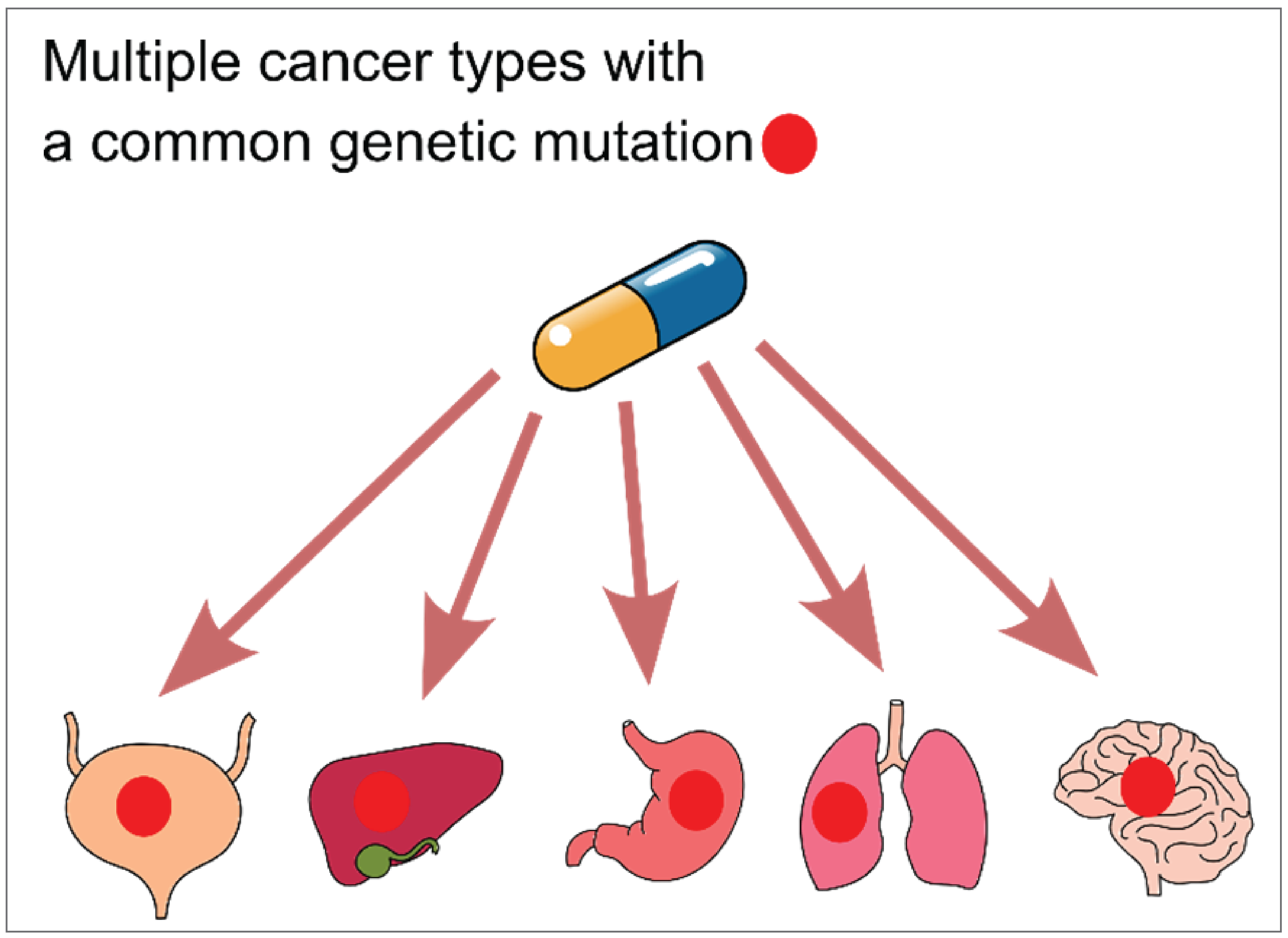
In this setting, a basket trial typically involves evaluating a single therapy targeting a group of patients who share a common clinical or genetic feature or biomarker, regardless of their histology type (Figure 1). One key feature of a basket trial is that the same outcome must be considered across all cohorts. Objective response rates are used as a common primary end point for each cohort in oncology, and the overall response rates for the full trial population are also typically estimated.

Heterogeneity in Basket Trials

The nature of basket trials, in which eligible patients with a common biomarker are recruited independently of tumour type, suggests there may be heterogeneity within tumour histology.⁴ One way to account for heterogeneity is to analyze each tumour type separately. However, sample sizes vary among cohorts, and studies for some cancer types — particularly rare ones — may suffer from poor recruitment and limited information on response rates. This could be related to the prevalence of the tumour type in the population, prevalence of the biomarker within the tumour type, or severity of the disease within this tumour type.³ Insufficient responses will likely lead to studies with limited power for some tumour types, and may fail to identify promising cohorts. Moreover, separate analyses of the cohorts will ignore the fact that different cohorts share a common biomarker and may react similarly to the same treatment. Allowing information to be shared between cohorts will likely increase the ability of the study to detect an effect, if an effect exists. For example, pooling all cohorts for the analysis and ignoring the potential heterogeneity will lead to a large gain in the efficiency of the study. However, this pooled analysis would assume the efficacy is the same across all cohorts, identical to the standard single-arm design. If there is significant heterogeneity among cohorts, a pooled analysis will lead to a biased treatment-effect estimate for each cohort. In addition, the pooled analysis has the potential to miss a true treatment effect when the treatment is only effective in some cohorts but ineffective or harmful in others. Thus, both complete pooling (which assumes homogeneity across all cancer types) and separate analysis (which assumes complete independence) are not generally preferred for basket designs.

A BHM can be used to address heterogeneity among cohorts and allow information-borrowing across cohorts by assuming treatment efficacy in different cohorts sharing a common parameter (i.e., the mean efficacy across cohorts varies based on some variation parameter).^2,7 Compared with analyzing all cohorts separately, a BHM increases the precision of the estimates while reducing the chances of obtaining extreme treatment-effect estimates in baskets with few patients. Crucially, BHMs use the data from a study to understand the appropriate level of pooling (depending on the observed similarity between the outcomes and under distributional assumptions around the mean treatment efficacy).

Overview of BHM

An Introduction to Bayesian Methods

Bayesian methods are an alternative to the more commonly used frequentist methods for statistical inference. Broadly, Bayesian methods define probability as expressing a degree of belief in an event. This contrasts with the frequentist interpretation, which defines probability as the frequency of an event in a long run of identical experiments. In practice, Bayesian inference requires 2 elements:

• a likelihood, which defines how the collected data are generated and the sense in which they are related to the parameters of interest; this element aligns with the frequentist approach to inference and is usually based upon standard statistical models like a generalized linear model, normal distribution, or Weibull distribution²⁴

• a prior distribution, which defines the investigator’s beliefs about the value of the model parameters before the data are collected.²⁵ Priors can be classified into 3 categories (based on the level of informativeness or degree of uncertainty around the parameter): informative, weakly informative, and diffuse. The classification depends on the context of the research question and the data that are being analyzed.²⁶ A diffuse prior, also known as a flat prior, reflects a complete lack of certainty about the parameter, whereas an informative prior reflects great certainty.

These 2 elements are then combined via Bayes’s theorem to estimate the posterior distribution for the model parameters, which summarizes all the information about the model parameters and is used as the basis of all inference. Crucially for HTA, a Bayesian analysis provides the complete joint distribution of the model parameters and can be used directly as input to a probabilistic analysis.⁸ Conversely, the posterior distribution can be summarized using standard metrics such as the mean, median, standard deviation (SD), and credible intervals (CrIs).²⁹ CrIs are the Bayesian equivalent to confidence intervals and are constructed such that there is a defined posterior probability that the model parameter lies within that interval.

Bayesian methods are commonly used in HTA, as the natural interpretation of findings makes the methods attractive, particularly as a vehicle for probabilistic analysis.^8,9 Bayesian methods specify a model for data collected in a study and a prior distribution for the parameters of this model. The prior distribution summarizes the information available about the model parameters before the data are collected. A Bayesian analysis then summarizes the updated knowledge on the parameters by balancing between the prior and observed data. The advantage of integrating prior information (e.g., information obtained through expert elicitation) into the analysis is that it allows for analyses when limited information is provided through the observed data, which can support decision-making.

BHMs have also been used in HTA in the context of patient-level cost-effectiveness analyses, as BHMs can be used to analyze multi-institutional cost and effectiveness data, or data originating from cluster randomized trials.¹³ The use of Bayesian methods in general in the context of patient-level cost-effectiveness analyses offers additional advantages related to addressing missing data. Finally, Bayesian approaches have been proposed for the purpose of conducting value of information analyses¹⁴ and for synthesizing information from single-arm trial data and retrospective data.¹⁵ More information about Bayesian methods can be found in van de Schoot (2021).¹⁰

BHM Model Specification

As discussed in the previous section, basket designs typically assume response rates as the primary outcome; more specifically, the response rate of different cohorts and the overall response rate are both of interest. Therefore, instead of assuming responses are identical across all cohorts, a BHM estimates the response rate of different cohorts by borrowing information across cohorts using a pooled response rate and the observed variance between the different cohorts. This model requires an assumption of exchangeability, so that the treatment effect can be considered as coming from the same distribution. Exchangeability means the sequence in which the cohorts are observed does not affect the assessment of the population effect, and it is a common assumption of statistical analyses (it can be thought of as a Bayesian equivalent of independent and identically distributed data).³⁶ A potential advantage of a BHM is that it allows predictions of the response rate of a new cohort or cancer type in a basket study, which is discussed further in the sections that follow.

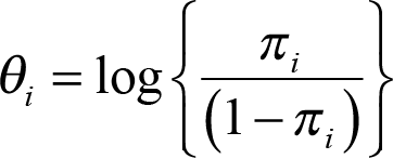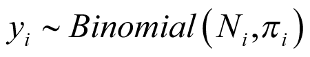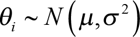
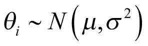
To formalize the modelling for a BHM, let be the probability of treatment response for cohort . If a logistic model is used, this can be linked to the parameter of interest as , where is the log odds of treatment response. The observed number of responses follows a binomial distribution , where is the number of patients in cohort . The BHM assumes that the parameter of interest follows a normal distribution with an unknown mean , which is the (log odds of) pooled response rate across all cohorts, and variance , which represents the variability in response across the different cohorts:

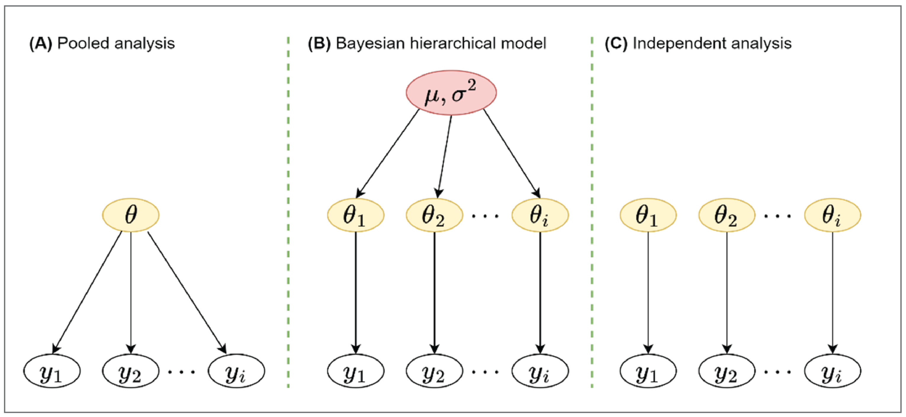
The unknown parameters and are at the second level (hierarchy) of distribution and are often termed hyperparameters as depicted in Figure 2 (part B). In hierarchical modelling, the priors are not specified directly. Instead, the prior distribution depends on other parameters, referred to as hyperparameters. A prior distribution is placed on those hyperparameters, referred to as hyperpriors, so the data can be used to update their values and provide inferences for them. The hyperparameter can be viewed as the distribution of the response rate in the overall population of cancer types, with the response rate in each cancer type corresponding to a random draw from this distribution.

Choosing the Prior for the Hyperparameters

Typically, a weakly informative prior for with a mean close to null effect is selected for . A flat prior — often a normal distribution with a large variance, or any other distribution with a long tail — might be employed. In the case of the normal distribution, the variance is more important than the mean. The choice of prior for is a critical aspect of the BHM, as it plays an important role in determining the shrinkage (i.e., the level of pooling between cancer types). In the 1 boundary of its space, when , the model collapses to complete pooling. This will ignore all of the variation between cohorts, as depicted in Figure 2 (part A). All of the cohorts are sampled from the same population and share a common parameter . In the other extreme, when approaches infinity, there is no borrowing, and the model is similar to independent analysis, as depicted in Figure 2 (part C). This means that cohorts are sampled from different populations and different cohorts have independent parameters . The BHM can be thought of somewhere in between a pooled analysis and an independent analysis, where the estimated response probability in each cohort is shrunk toward the estimated population mean . This is a safeguard to avoid extreme estimation if limited sample sizes are available in some cohorts. The estimated population mean will then be pulled toward the cohorts with larger sample sizes, if compared against independent analyses.

Based on the interpretation of in the previous paragraph, it can be noted that the results from a BHM are sensitive to the selection of a prior for . Thus, the prior should be carefully selected with a reasonable rationale based on the between-strata heterogeneity. In BHMs, it is recommended to avoid a prior that suggests that is too close to zero, as this forces the results to be too close to a pooled analysis. One distribution that can provide good results is a half-t family prior.³⁷ The degrees of freedom increase the certainty of the half-t distribution, but the scale increases the uncertainty. A weakly informative uniform prior on the SD has also been suggested by other studies.³⁸ However, it should be avoided when the number of cancer types is small (e.g., 5). The uniform prior truncates the parameter space as discussed in the previous section and should be avoided for this reason. Another potential distribution for the prior is the inverse gamma family, but the final results are very sensitive to the parameters of the inverse gamma distribution when the number of cancer types is small.³⁷

Figure 2: Graphical Presentation of Pooled Analysis (A), Bayesian Hierarchical Model (B), and Independent Analysis (C)

Prediction of New Cancer Type

It may not be possible to recruit all cancer types in a study, even when the molecular subtype is present. This is problematic in an HTA context, where components such as economic evaluations require the consideration of all possible populations affected by a decision. Given that basket trials are used predominantly to inform decisions that extend beyond observed cancer types, extrapolation of inference might be possible for unobserved cancers, conditional upon strong assumptions. A BHM can, in principle, allow for the prediction of the response rate of a new cancer type, even if it is not included in the basket study. The uncertainty of response rate will account for the sample size of the study, the information borrowed across cancer types, and the heterogeneity across different subtypes. This is because, for a new cancer type that is not presented in the study, the parameter of interest

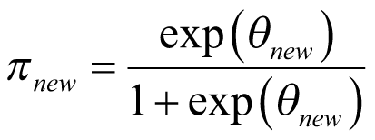
(predicted response rate of the new cancer type) can be obtained as follows:

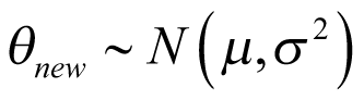
where and are both estimated from the posterior distribution, conditional on the data from the study and the weakly informative priors, and are subject to uncertainty. From this distribution of , the response probability of this new cancer type can be derived as:

This prediction may be reasonable if the expected response of the new cohort falls within the range of the observed rate of response and if the expected response is deemed clinically valid. In particular, it would be necessary to provide reasonable historical evidence for the similarity of the new cancer type to the observed cancer types, in terms of the response rate.

The fact that BHMs allow for a statistical prediction of expected response in a new cancer type, with uncertainty, does not necessarily suggest that the preferred approach in an economic evaluation is indeed directly using the predicted response as input. For example, the model could incorporate pessimistic priors as a means to add skepticism and perhaps reduce the expected response rate in the unobserved cancer types.

Different Types of BHMs

Previously, BHMs have been criticized, as they may not be appropriate to borrow information across all cancer types by assuming that all cancer types are similar (known as the full exchangeability assumption).³⁹ Consequently, different types of BHMs have been proposed to borrow information only between similar cancer types. The exchangeability-nonexchangeability (EXNEX) model is an extension of the BHM, introducing a nonexchangeable component.⁴⁰ It allows for some cancer types to be exchangeable, and also includes a nonexchangeable component containing independent types. The data and appropriate weights with some justifications are used to determine which component a cancer type belongs to. It has been suggested that nonextreme weights should be used such that exchangeability and nonexchangeability are a priori likely; for example, both the exchangeable and nonexchangeable component should have the same weight and must be summed to 1.⁴⁰ The treatment effects are not fully exchangeable in this model, and the predictive distribution will differ for some tumour types. Therefore, it is harder to predict the response rate of a cancer type that was not included in the study. The EXNEX model has been proposed as an alternative to the BHM in the analysis of basket trials, although its use in practice has so far been limited.

Other models accounting for heterogeneity in response rates may be in the form of a clustered Bayesian hierarchical model (CBHM), aiming to categorize similar cancer types into clusters or subgroups.^41-44 The determination of subgroups varies by model, but the general principle of a CBHM is that treatment effects are assumed to be independent between clusters but exchangeable within subgroups. If the clusters are predefined, the approach is similar to analyzing multiple independent BHMs without borrowing information from other cancer types outside the subgroup. The prediction of new cancer types can be made for each subgroup separately, and a decision should be made to determine the subgroup in which a new cancer type belongs.

Figure 3: Graphical Presentation of EXNEX Model With 2 Exchangeable Components and 1 Nonexchangeable Component (A), and CBHM With 3 Subgroups (B)

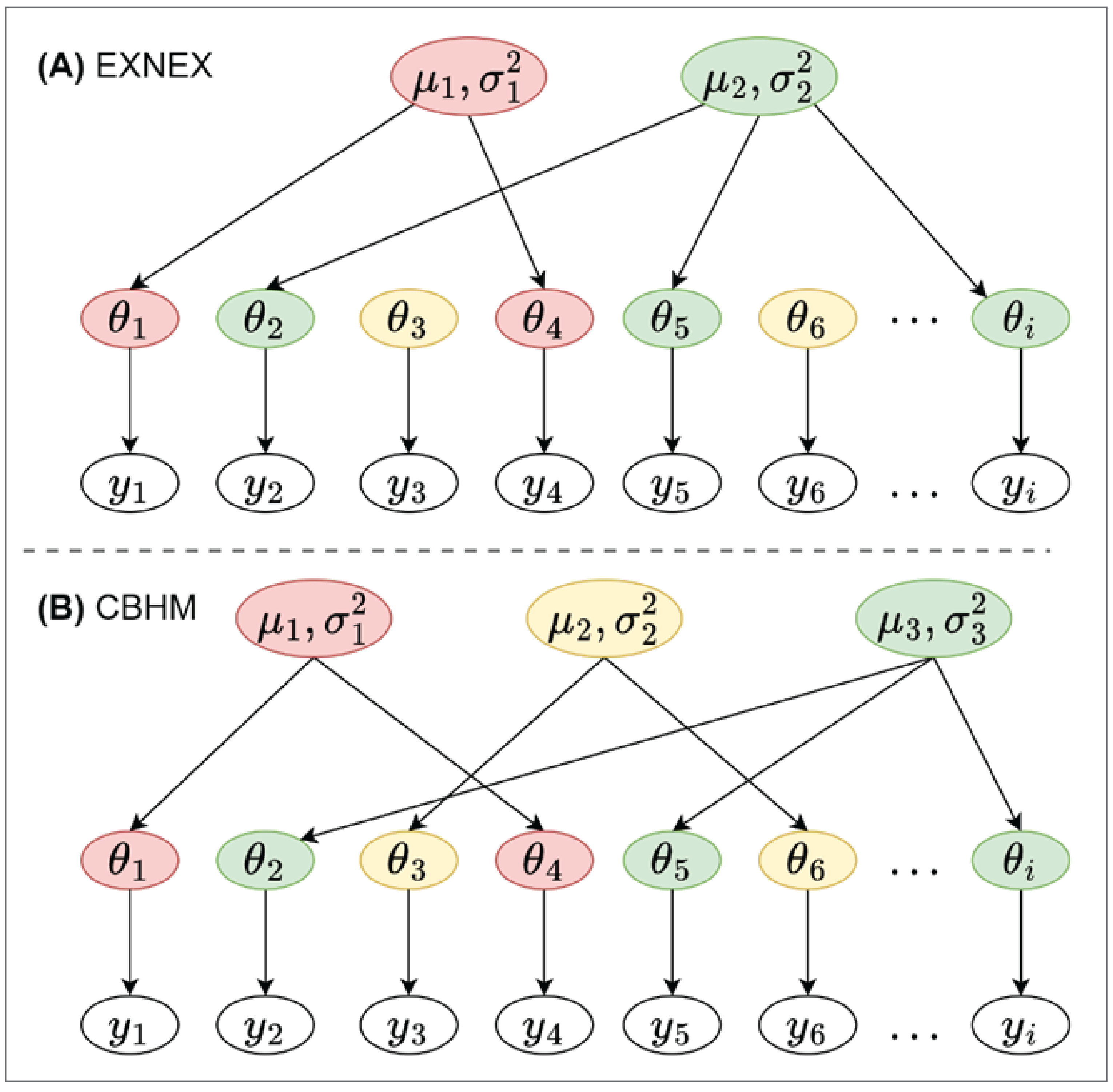
EXNEX = exchangeability-nonexchangeability; CBHM = clustered Bayesian hierarchical model.

Placing BHM and Basket Trials in the Context of the Economic Evaluation

The heterogeneity between and limited information within cancer types in basket trials create additional challenges in health economic evaluation. Different cancer types will not only benefit differently from the treatment but the benefit, as measured in the basket trials, can have different impacts on the health outcomes that matter most in health economics: length and quality of life. For example, a response rate of 50% in patients with metastatic urothelial cancer might not have the same impact on survival as the same 50% response rate in patients with a less deadly cancer (e.g., colorectal). In addition, comparator treatments are likely to be different between cancer types, thereby making any approach inapplicable when it assumes a pooled economic analysis that ignores heterogeneity between cancer types. Finally, policy-makers might choose to consider the fact that effectiveness and cost-effectiveness differ between cancer types, and issue different recommendations for different cancer types. This provides an additional argument for the analysis and presentation of cost-effectiveness by cancer type, perhaps in addition to an overall estimate.

In health economic evaluation, cost-effectiveness is usually assessed with data from randomized controlled trials in terms of overall survival (OS) and quality-adjusted life-years (QALYs). Estimating cost-effectiveness is challenging in the presence of limited follow-up, because the time-to-event (TTE) data are immature. Estimation of long-term survival is further complicated in cases where the primary outcome is an intermediate (or surrogate) outcome such as response rate. In such cases, prediction models are typically used to connect long-term TTE outcomes with response rates. Response-based end points are commonly used in cancer studies because they occur faster, reducing the need for lengthy clinical studies. While response-based end points may be a poor surrogate for OS, they represent the most commonly used primary end point in basket trials. A National Institute for Health and Care Excellence (NICE) appraisal reviewed response rates as surrogate end points for OS and summarized 4 main methods to quantify the relationship between response rate and OS:¹⁸ a meta-analysis–based approach, landmark response framework, risk prediction model, and BHM.

The relationship between response rate and OS reported in a different real-world study or meta-analysis study may be used to extrapolate the OS. However, the population used in such studies may not match well with the study population in the basket trial. An alternative approach is to use the landmark response framework, which assumes that response is a perfect surrogate end point for OS. Here, OS varies by response but is common across cancer types. A risk prediction model can be used to estimate OS based on patients’ characteristics, including response status. However, this method may have the same drawbacks as the meta-analysis–based approach. The NICE review suggests that response rate is not a reliable surrogate end point for OS, and there is no clear relationship between response and OS. Although an appropriate BHM can be applied to TTE outcome data, a short time horizon will likely lead to substantial uncertainty and unstable estimates. To date, the majority of basket trials do not use a BHM in the analysis of OS or progression-free survival, largely due to limited sample size.

Handling Uncertainty

The incorporation of BHMs in economic evaluations involves some of the challenges and benefits associated with the use of BHMs in a (network) meta-analysis. Ideally, a BHM pairs best with an economic evaluation model that is fully probabilistic and uses the full joint posterior of the efficacy parameters from the BHM. This allows for the seamless estimation of the posterior distribution of the cost-effectiveness outcomes and the full propagation of parameter uncertainty. Using the same approach for the clinical and health economic model also allows for a more thorough investigation of the impact of the prior distributions on the cost-effectiveness outcome. Finally, using the same framework would make drawing expected effectiveness for cancer types that are not part of the basket trials simpler, because the posterior distribution of the overall effect would be used directly as input in the simulation.

Output of BHM analyses could be incorporated in models that are built external to the analysis; however, it is important to note that, because a BHM implicitly assumes some relation between the cancer types, the parameters specific to the cancer type are likely to be correlated. Therefore, this correlation structure on the parameters needs to be propagated to the economic model. The most appropriate way for that to be done is to extract the values from the posterior parameter distributions as estimated from the BHM and use them as input in the economic model. In other words, in a probabilistic analysis, each iteration would sample — without replacement — from the values drawn from the joint posterior distributions or response rates estimated from the BHM. The posterior distributions from the BHM account for the uncertainty of the parameters and correlation among parameters. Propagating each realization of the posterior distribution in the economic model will enable obtaining of the full distribution of the decision-making process.⁴⁵ Alternative approaches exist (e.g., sampling from the marginal distributions of response), although these methods have been shown to misrepresent uncertainty, especially in situations where borrowing of information between cancer types is extensive. Some guidance on propagating uncertainty from BHMs is offered in the network meta-analysis literature.⁴⁶

Practical Considerations When Appraising the Use of Evidence From Basket Trials in Economic Evaluations

When appraising the evidence from an economic evaluation that is based on a BHM, there are a number of considerations: generalizability, comparator selection, how costs are incorporated, and the use of survival extrapolation beyond the period of the trial evidence. The strength of the underlying trial evidence and the methods used to integrate it into the economic model have a meaningful effect on the level of uncertainty surrounding the model’s estimated costs and outcomes. Each of these aspects are discussed in this section. For researchers and analysts, a list of the specific items to consider when conducting and/or appraising an economic analysis that incorporates a BHM has been included in Appendix 2.

Generalizability

The projection of the evidence derived from a basket trial represents a key consideration in the appraisal. The issues about the generalizability of the evidence are likely affected by the population and cancer types included in the study and the modelling method used in the analysis, and these 2 issues are discussed subsequently.

Population and Cancer Types

In basket trials, the population included in the trial does not reflect the general population, because the distribution of the biomarker varies between cancer types. The distribution of the cancer type and number of patients in each cancer type should match the target population with the same biomarker; however, this is challenging because the cancer type distribution varies between trial sites (e.g., some sites have more patients with a breast cancer diagnosis, but others have more lung cancer diagnoses).

Adjusting for these types of bias as part of the health economic evaluation may be challenging. Simple approaches that have previously been proposed would be to assume that the cost-effectiveness is the same across cancer types, or to assume that the distribution of cancer types in the trial is representative of the licensing population.¹⁸ The former assumption is very unlikely to hold, because different cancer types have different comparators with different costs and outcomes. Although the latter assumption may seem more reasonable, the propriety of this assumption is difficult to test in practice. Bias would be expected if there are discrepancies in cancer type distribution between the trial population and the target population. The direction and magnitude of such bias is also difficult to assess because information on the prevalence of a biomarker or genetic characteristic is often scant and not specific to jurisdictions for which decisions are being made. Adjustments based on reweighting the trial population to reflect the licensing population could be a reasonable option, especially as evidence on genetic markers becomes more widely available.

Different study designs have been proposed to increase the efficiency of a study. Adaptive designs may drop cancer types characterized as ineffective at an early stage. Alternatively, some cancer types might be dropped from an analysis due to limited information, possibly due to very small sample sizes. Such actions are likely to affect the target population and the evidence raised from the study will no longer apply to all other cancer types with the same biomarker. One consequence would be to constrain the decision exclusively to the study cancer types included in the final analysis. The alternative in which a best guess of treatment efficacy is applied for the cancer types for which no evidence exists would allow for inference on a more correct population, but would have greater uncertainty.

Extending the evidence from a study population to unobserved cancer types is a key consideration, especially for the approval of cancer types with the same biomarker that were not included in a study. It is important to consider the uncertainty around the efficacy prediction of the unpresented cancer type. Moreover, there might be reasons that some cancer types are not included in a study, possibly related to the cost of a test, prevalence of a biomarker, and cancer types among the population or the expected treatment efficacy for that biomarker. It is not reasonable to extrapolate evidence from only 3 or 4 cancer types to all cancers. Nevertheless, there is no consensus on how many cancer types are needed to extend the evidence to all cancer types. These factors should be considered during the evaluation of the cost-effectiveness of a treatment in unobserved cancer types. Extensive sensitivity analyses should be conducted in which extreme assumptions are made on the effectiveness for these unobserved cancer types.

Modelling Method

Heterogeneity in the treatment effect between cancer types is a critical issue in basket trials. To illustrate the impact of potential heterogeneity in efficacy and health economic evaluation estimates, a case study is presented in Appendix 1 in which the BHM was applied to trial response data. This case study illustrates that response rates can vary widely between cancer types.

When clusters of cancer types with similar characteristics exist, then the default BHM may not be an appropriate vehicle for borrowing information across cancer types, as it assumes that all cancer types are similar. Various statistical methods have been proposed to borrow information only from cancer types that react similarly. They include models that categorize cancer types into clusters and borrow information only within the group or use weighting methods to borrow more information from a similar cancer type and less from a dissimilar one. The similarity is determined by data or expert knowledge. These methods, including but not limited to EXNEX and CBHM, may improve the precision of the estimation and statistical power, especially in baskets with a large number of cohorts. However, the results of these methods are harder to interpret. The exchangeability no longer applies to all cancer types, and it is not feasible to assume the predictive distribution represents the unpresented tumour types. The generalizability issues raised from these methods should be carefully considered when appraising the economic evaluation.

Comparator

Most basket trials are a collection of single-arm studies and do not contain a control arm. An appropriate comparator is required for economic evaluations. The historical control method used in single-arm studies may suffer from bias due to differences between current and historical patients. For example, treatment efficacy may increase as clinical care improves over time. Finding a good comparator is more challenging in basket trials because the historical data typically lack biomarker information used in basket trials to differentiate between cancer types. It is difficult to find a single data source that covers all cancer types with a specific biomarker. Selecting a proper comparator from multiple data sources for different cancer types will aggravate selection bias. It is also possible that no data will be available for some cancer types. In such cases, the possible bias and uncertainty introduced in the model due to inappropriate comparators need to be assessed through sensitivity analyses.

Patients in historical controls may have characteristics that differ from those in the trial. One would need to consider matching the patients’ characteristics with the treatment arm and keep the internal validity, or decide that the historical controls ought to reflect the target population and aim for external validity. Conceptually, the latter is more in line with the requirement of developing guidance after consideration of a real-world treatment effect. However, if the distance in confounding characteristics between the treatment population and the target population is large, then the potential for bias is large. Using historical controls as a comparator is more difficult if the common biomarker used in the basket trial has prognostic effects itself, or association with other prognostic factors, especially if the prognostic effect varies across cancer types.

Other methods, such as population-adjusted indirect comparison using observation data as a comparator, have been proposed. These methods include matching-adjusted indirect comparisons and simulated treatment comparisons, and have been previously used in CADTH submissions. The NICE guidance website contains a comprehensive review on sources and synthesis of evidence methods. Although these methods can be used in basket trials, finding studies that match the trial population may be challenging. Despite the limitations of these methods, assumptions of this kind could generate a reasonable comparator, under stringent assumptions.⁴⁷

Alternatively to the methods described previously, using nonresponders as a proxy of patients not receiving active treatment in a trial has been proposed.⁴⁸ With this method, the TTE outcomes are based on observed nonresponders, assuming the comparator does not achieve a disease response, meaning that no effective treatment exists for the disease. The comparator will share the same characteristics in the study. However, this method assumes that the TTE outcomes are fully explained by response status or that tumour response is a perfect surrogate end point for the TTE outcomes. This is not always the case, as some patients still benefit from the treatment without a tumour response.

Most of the proposed work to construct a comparator as described in this section requires similarity of the historical control data. The population's heterogeneity creates significant challenges in creating a proper comparator. No methods have shown a conclusive advantage over others. Utilizing different approaches may help to understand the uncertainty around the evidence. To further support the decision-makers, understand the robustness of the method, the E-value and threshold analysis were proposed.^49,50 Threshold analysis quantifies the amount of change needed in the parameter to obtain different recommendations. The recommendation may be considered robust if the amount of change is considered implausible. The E-value functions the same way to inform the robustness of the evidence. The heterogeneity and difference between trial population and general population due to the common biomarkers should be accounted for when applying those approaches.

Costs

Because basket trials target populations with a certain biomarker of genetic characteristics, it is important for health economic evaluations that rely on basket trials to incorporate the cost of testing for that biomarker or characteristic. The costs may vary depending on the testing strategy, the sensitivity of the testing method, and the frequency of the biomarker in each cancer type. The frequency of a biomarker varies across cancer types and has a significant impact on the number of patients needed to be screened. Biomarkers with low frequency in particular cancer types increase the cost of finding eligible patients for the treatment. For example, common cancer types with small positive biomarkers will increase the eligibility checking cost and cost of testing may attribute a significant portion of the costs associated with the economic evaluation. It is not reasonable to apply 1 cost to all cancer types without considering the variability of the frequency of a biomarker across cancer types. Availability of such testing procedures may also differ between experimental settings and routine practical use.

Biomarker frequency varies by cancer type and some cancers may be excluded from a study due to a lack of eligible patients. This may increase the cost of finding eligible patients and should be considered when estimating the cost-effectiveness of unpresented cancer types. Reports should include the number of patients screened in each cancer type, including on the unobserved cancer types, as well as the number of patients who tested positive for the biomarker to inform the prevalence of the biomarker in each cancer type.

Survival Extrapolation

Economic evaluation of oncological therapies typically requires the estimation of survival probabilities over a patient cohort’s full lifetime. Extrapolating survival beyond the study period and accounting for cancer type heterogeneity may be potentially challenging due to a basket trial's limited follow-up period and the inherent heterogeneity present. Extrapolation from immature TTE outcomes may lead to highly unstable estimates. Given that patients with different cancer type diagnoses experience different natural history trajectories over time, survival varies across cancer types. It is not appropriate to fit a single model to the overall population without accounting for heterogeneity between cancer types, unless there is very clear evidence of the absence of heterogeneity between cancer types. It should be reminded that the absence of evidence of heterogeneity (e.g., a low with wide CrIs) does not imply evidence of the absence of heterogeneity.

Standard parametric survival models are typically used in economic evaluations to extrapolate survival beyond the study period by adopting appropriate assumptions on the survival shape after the study period.⁵¹ Flexible survival models with spline functions may fit the data well, but they reduce to standard and possibly oversimplistic parametric models after the observation period. An alternative fractional polynomial will place no restriction on survival beyond the observed data but may lead to implausible predictions.⁵² In addition, small samples within cancer types make estimation of parametric models unstable, with consequences on the extrapolations beyond the observed survival period. The challenge is greater when attempting to fit more flexible survival models (e.g., spline or multiparameter models). A guideline regarding the selection of the survival model in the context of health economic evaluation of immune therapy has been published recently.⁵³ This guideline provides an algorithm to aid model selection.

In addition to the inherent problems of extrapolating survival beyond the study time horizon, heterogeneity between cancer types is another challenge in the cost-effectiveness analysis of basket trials. Including cancer type as a covariate to account for variation between cancer types in 1 or more of the parameters of an assumed distribution is unlikely to help with small sample size, as this would impose additional assumptions in the modelling approach (e.g., proportional effect of cancer type on hazards). Also, this method may not provide information on the unobserved cancer types. To account for heterogeneity, a mixture model with 2 or more components may be used, but the performance of such models in survival extrapolation has not been assessed.

Another limitation associated with survival extrapolations from basket trials relates to the nature of the outcomes used. As mentioned previously, basket trials often rely on response rates as the primary outcome. However, the 2 most common models used in economic evaluations of oncological interventions (partitioned survival models and state-transition models) require estimates of survival or transition probabilities to simulate cohorts across health states. Extrapolating response rates to survival outcomes requires an additional step. Although the validity of objective response as a surrogate end point of OS remains questionable and may not be reliable, a surrogate-based model accounting for relevant uncertainty might be preferable over the immature survival data. In this step, the analyst needs to make an assumption regarding the predictive relationship between response rates and survival.

One approach is to assume that response is essentially a perfect surrogate for TTE outcomes in response-based landmark models. They explicitly model responders and nonresponders in each cancer type separately. This method is well suited for basket trials, but selecting the landmark time point and uncertainty is challenging. Moreover, this approach may also suffer from a short study time horizon and small sample sizes.

Another approach is to use meta-analysis to predict the relationship between the surrogate end point and OS. However, it may be difficult to find studies with the same biomarkers, and the studies included in the analysis may not correspond to the underlying population of the study. Additionally, it is important to consider the appropriateness of the model used to associate the relationship. The bivariate random-effects meta-analysis model and other extensions can borrow information across studies, and accounting for the uncertainty surrounding the relationship within a Bayesian framework would be more appropriate in this situation.^54,55

BHMs for survival data, like response outcome analyses, can investigate heterogeneity in TTE outcomes.⁷ The models allow for survival distributions with different rate parameters across cancer types and those parameters may shrink across cancer types, facilitating borrowing of information. However, such models also suffer from short time horizons and small sample sizes within cancer types, while exchangeability of latent parameters is harder to test. Examples of BHMs for survival data are rare, especially within the context of basket trials.

Discussion

There is an increasing use of basket trial designs, specifically for some oncology technologies. The heterogeneity among cancer types, limited sample sizes, lack of comparators, and use of surrogate end points pose challenges when considering the application to economic evaluations. Based on this document, a well-designed analysis borrowing information across cancer types will provide useful information, given the limited information for each cancer type but also the conceptual and practical limitations of pooling across all cancer types.

CADTH requires a stratified analysis without information-borrowing to be performed as a supplement to the analyses using the BHM approach. The guidelines outlined in this report should be supplemented by the relevant CADTH guidelines, including but not limited to Guidelines for the Economic Evaluation of Health Technologies: Canada (Fourth Edition), Specific Guidance for Oncology Products, and Guidance for Economic Evaluations of Tumour-Agnostic Products.

Challenges

Finding an adequate comparator is critical for health economic evaluation if the basket trial is single-arm and there is an absence of randomization. Although several approaches were mentioned in the preceding section, it is difficult to select 1 method that fits all circumstances.⁵⁶ This is especially true when the trial population comprises multiple cancer histologies that share a particular biomarker. It is advised that several approaches with complimentary weaknesses and strengths be used. Other methods, including threshold analysis and E-values, may help the reviewer to understand the robustness of the evidence. A basket trial with a control arm and randomization is preferred when feasible.

The prevalence of a biomarker in different cancer types, as well as recruitment, may change the distribution of cancer types in the trial population. If the trial population's distribution differs from that of the target population, the evidence obtained from the trial population may not apply to the target population. It is critical to fully assess the disparity between the trial and the target populations, and such differences must be effectively accounted for.

Evidence raised from the population may indicate the treatment is cost-effective for some cancer types but not others. Recommendation of the treatment to non–cost-effective cancer types is not encouraged unless there is enough evidence to do so. Even with carefully planned data collection, a basket trial may contain only a subset of eligible cancer types. BHMs offer a vehicle to estimate the distribution of treatment effect in the target population and predict the treatment effect for cancer types not included in the study. The generalizability of the evidence raised from the study to unobserved cancer types is closely tied with discrepancies between the study population and target population, number of cancer types included in the study, exchangeability of the unobserved cancer types with cancer types included in the study, and sample size. If a decision is to be made in this situation to unobserved cancer types, evidence should be carefully evaluated and not encouraged for recommendation unless there is enough evidence to do so or unless more evidence has accrued. As demonstrated in our real-world example (Appendix 1), extending such predictions to unobserved cancer types tends to be highly uncertain with wide CrIs.

To improve the efficiency of the design, different mathematical and statistical methods have been proposed for different trial purposes. As described in the Different Types of BHM and Generalizability sections, most methods focus on borrowing information only from similar cancer types. With such assumptions in mind, different BHM extension methods for basket trials have been developed recently.⁵⁷ Sharing information is only valid if the common biomarker is a treatment prognostic factor, which is difficult to verify in practice.⁵⁸ In most of the proposed methods, the similarity across baskets is based on response rate alone, which may not work well, especially when only a few patients are available. Incorporating clinical biomarker information into cluster similar baskets has also been proposed,⁵⁹ but including such biomarkers could be challenging to justify in practice. While researchers may prefer a complex model, the choice of such a model introduces additional methodological challenges and results may be difficult to interpret. The introduction of new assumptions also generally means additional uncertainty due to spreading the data thinner. Challenges arise in justifying the assumption of interchangeability across all cancer types and in generalizing the evidence to unobserved cancer types when certain cancer types are dropped during the conduct of the trial due to poor outcomes or when information is shared within clusters of similar cancer types. As mentioned previously, the creation of clusters complicates predictions for unobserved cancer types, as it requires classification of these cancer types to clusters before prediction.

Beyond heterogeneity in the treatment effect, baseline heterogeneity should be acknowledged and reflected in the economic evaluation when appropriate. Survival data can be used in the health economic evaluation with a careful selection of the survival model based on existing guidelines.⁵³ Due to the immaturity of TTE outcome data in basket trials, a surrogate end point might be used in health economic evaluations. A tool has been developed to support the use of surrogate end points in health economic evaluations.⁶⁰ Although the validity of the relationship between the surrogate end point and the TTE outcome remains unclear, a carefully designed surrogate end point–based model is preferable to a heavily censored TTE outcome. The uncertainty surrounding the relationship between the surrogate and TTE outcome should be examined in the modelling process (e.g., through a “worst-case scenario” analysis). A meta-analysis–based approach is recommended to reflect the relationship between the surrogate end point and the TTE outcome, but mature TTE outcome data should be used when feasible.

Further Research

The field of BHM for the analysis of basket trials is still evolving. For example, novel methods are proposed where cancer groups within baskets are formed without the need to be specified a priori, unlike models like EXNEX would require. Novel basket trials designs are proposed that will likely warrant further exploration with regards to their integration in economic evaluations.⁶¹ For example, the “basket of baskets” design considers a case where genetic testing of the tumour happens and then the patient is allocated to a different basket trial based on the results.

There is considerable uncertainty with regards to best practices in incorporating cancer type evidence in OS and progression-free survival (PFS) directly from basket trials. On the 1 hand, methods that rely on the relationship between response and survival rely on strong assumptions of predictability and association. Further, any survival end points from basket trials will likely be immature and largely underpowered for cancer type–specific analysis. Additionally, some of the therapies assessed in basket trials are intended to be curative, which might require more flexible distributional assumptions when modelling survival probabilities. More work to evaluate the relative advantages of these approaches is needed.

International efforts are under way to collect information in biobanks and retrospective registries with tumour information (i.e., retrospectively genotyping tumour samples to assign genetic characteristics). These efforts could eventually increase the availability of real-world evidence that can provide comparators in such single-arm studies. Although using real-world evidence to form a synthetic control for single-arm studies requires strong assumptions that are unlikely to hold in many such applications, the presence of biomarker or genetic marker information in the population will make such comparisons plausible. It must be noted that it is unlikely that these methods will adhere to these strict assumptions regardless of the presence of biomarker information in the data.

Owing to the uncertainty in health economic evaluation in basket trials, treatments that are considered cost-effective based on the primary analyses and expected incremental cost-effectiveness ratios may often have a high risk of not being cost-effective. Sources of uncertainty in these cost-effectiveness models stem from the wide range of assumptions required to perform an economic evaluation, the sample size of the underlying basket trial that forms the basis of the efficacy data for the evaluation, and other modelling assumptions. The use of both sensitivity analyses and value of information analyses can provide a useful framework for decision-makers to understand the impact of this uncertainty on their decisions.^14,45

Conclusion

As new research approaches generate new kinds of clinical evidence, HTA agencies need to understand how best to incorporate it into decision-making. Economic evaluations are a key component of HTA, and typically rely on models to translate clinical evidence into an estimate of the impact that adoption decisions will have on patients and the health care system. This report has described the way that basket trials allow researchers to observe the common effect of treatments across a variety of tumour types, and how BHMs allow for the evidence generated by these trials to be incorporated into economic analysis. While these methods are still associated with a high degree of uncertainty, this report highlights some specific approaches to understanding and characterizing that uncertainty, so that HTA agencies like CADTH can properly incorporate research findings from high-quality basket trials as they seek to ensure that patients have timely access to innovative therapies that provide good value to the health care system.

References

1.Park JJH, Siden E, Zoratti MJ, Dron L, Harari O, Singer J, et al. Systematic review of basket trials, umbrella trials, and platform trials: a landscape analysis of master protocols. Trials. 2019 Sep 18;20(1):572. PubMed

2.Berry SM, Broglio KR, Groshen S, Berry DA. Bayesian hierarchical modeling of patient subpopulations: Efficient designs of Phase II oncology clinical trials. Clin Trials. 2013 Oct 1;10(5):720–34. PubMed

3.Park JJH, Hsu G, Siden EG, Thorlund K, Mills EJ. An overview of precision oncology basket and umbrella trials for clinicians. CA Cancer J Clin. 2020;70(2):125–37. PubMed

4.Haslam A, Olivier T, Tuia J, Prasad V. Umbrella review of basket trials testing a drug in tumors with actionable genetic biomarkers. BMC Cancer. 2023 Jan 13;23(1):46. PubMed

5.Gaultney JG, Bouvy JC, Chapman RH, Upton AJ, Kowal S, Bokemeyer C, et al. Developing a Framework for the Health Technology Assessment of Histology-independent Precision Oncology Therapies. Appl Health Econ Health Policy. 2021 Sep 1;19(5):625–34. PubMed

6.Weymann D, Pollard S, Lam H, Krebs E, Regier DA. Toward Best Practices for Economic Evaluations of Tumor-Agnostic Therapies: A Review of Current Barriers and Solutions. Value Health. 2023 Nov 1;26(11):1608–17. PubMed

7.Thall PF, Wathen JK, Bekele BN, Champlin RE, Baker LH, Benjamin RS. Hierarchical Bayesian approaches to phase II trials in diseases with multiple subtypes. Stat Med. 2003;22(5):763–80. PubMed

8.Bayesian methods in health technology assessment: a review. Health Technol Assess [Internet]. 2000 Dec 11 [cited 2022 May 10];4(38). Available from: https://www.journalslibrary.nihr.ac.uk/hta/hta4380/ PubMed

9.Cooper NJ, Spiegelhalter D, Bujkiewicz S, Dequen P, Sutton AJ. USE OF IMPLICIT AND EXPLICIT BAYESIAN METHODS IN HEALTH TECHNOLOGY ASSESSMENT. Int J Technol Assess Health Care. 2013 Jul;29(3):336–42. PubMed

10.van de Schoot R, Depaoli S, King R, Kramer B, Märtens K, Tadesse MG, et al. Bayesian statistics and modelling. Nat Rev Methods Primer. 2021 Jan 14;1(1):1–26.

11.Laws A, Tao R, Wang S, Padhiar A, Goring S. A Comparison of National Guidelines for Network Meta-Analysis. Value Health. 2019 Oct 1;22(10):1178–86. PubMed

12.Jenkins DA, Hussein H, Martina R, Dequen-O’Byrne P, Abrams KR, Bujkiewicz S. Methods for the inclusion of real-world evidence in network meta-analysis. BMC Med Res Methodol. 2021 Dec;21(1):207. PubMed

13.Grieve R, Nixon R, Thompson SG. Bayesian Hierarchical Models for Cost-Effectiveness Analyses that Use Data from Cluster Randomized Trials. Med Decis Making. 2010 Mar;30(2):163–75. PubMed

14.Jackson CH, Baio G, Heath A, Strong M, Welton NJ, Wilson ECF. Value of Information Analysis in Models to Inform Health Policy. Annu Rev Stat Its Appl. 2022;9(1):95–118. PubMed

15.Dron L, Golchi S, Hsu G, Thorlund K. Minimizing control group allocation in randomized trials using dynamic borrowing of external control data – An application to second line therapy for non-small cell lung cancer. Contemp Clin Trials Commun. 2019 Dec;16:100446. PubMed

16.Tarride JE, Cheung M, Hanna TP, Cipriano LE, Regier DA, Hey SP, et al. Platform, Basket, and Umbrella Trial Designs: Issues Around Health Technology Assessment of Novel Therapeutics. Can J Health Technol [Internet]. 2022 Jul 6 [cited 2023 Mar 31];2(7). Available from: https://canjhealthtechnol.ca/index.php/cjht/article/view/nm0002

17.Haines A, LaPlante S, Lee K. Guidance for economic evaluations of tumour-agnostic products. Ott CADTH. 2021;

18.Murphy P, Glynn D, Dias S, Hodgson R, Claxton L, Beresford L, et al. Modelling approaches for histology-independent cancer drugs to inform NICE appraisals: a systematic review and decision-framework. Health Technol Assess. 2022 Jan 5;25(76):1–228. PubMed

19.Drilon A, Laetsch TW, Kummar S, DuBois SG, Lassen UN, Demetri GD, et al. Efficacy of Larotrectinib in TRK Fusion–Positive Cancers in Adults and Children. N Engl J Med. 2018 Feb 22;378(8):731–9. PubMed

20.Murphy P, Claxton L, Hodgson R, Glynn D, Beresford L, Walton M, et al. Exploring Heterogeneity in Histology-Independent Technologies and the Implications for Cost-Effectiveness. Med Decis Making. 2021 Feb 1;41(2):165–78. PubMed

21.Team R. Larotrectinib (Vitrakvi). Can J Health Technol [Internet]. 2021 Nov 12 [cited 2023 Mar 31];1(11). Available from: https://www.canjhealthtechnol.ca/index.php/cjht/article/view/pc0221r

22.Michels RE, Arteaga CH, Peters ML, Kapiteijn E, Van Herpen CML, Krol M. Economic Evaluation of a Tumour-Agnostic Therapy: Dutch Economic Value of Larotrectinib in TRK Fusion-Positive Cancers. Appl Health Econ Health Policy. 2022 Sep;20(5):717–29. PubMed

23.Suh K, Carlson JJ, Xia F, Williamson T, Sullivan SD. The potential long-term comparative effectiveness of larotrectinib vs standard of care for treatment of metastatic TRK fusion thyroid cancer, colorectal cancer, and soft tissue sarcoma. J Manag Care Spec Pharm. 2022 Apr 1;1–9. PubMed

24.Etz A. Introduction to the Concept of Likelihood and Its Applications. Adv Methods Pract Psychol Sci. 2018 Mar 1;1(1):60–9.

25.O’Hagan A, Buck CE, Daneshkhah A, Eiser JR, Garthwaite PH, Jenkinson DJ, et al. Uncertain Judgements: Eliciting Experts’ Probabilities [Internet]. 1st ed. Wiley; 2006 [cited 2023 Nov 14]. Available from: https://onlinelibrary.wiley.com/doi/book/10.1002/0470033312

26.Gelman A, Simpson D, Betancourt M. The Prior Can Often Only Be Understood in the Context of the Likelihood. Entropy. 2017 Oct 19;19(10):555.

27.Seaman JW, Seaman JW, Stamey JD. Hidden Dangers of Specifying Noninformative Priors. Am Stat. 2012 May 1;66(2):77–84.

28.McNeish D. On Using Bayesian Methods to Address Small Sample Problems. Struct Equ Model Multidiscip J. 2016 Sep 2;23(5):750–73.

29.Robert CP, Casella G, Casella G. Monte Carlo statistical methods. Vol. 2. Springer; 1999.

30.Geyer CJ. Markov Chain Monte Carlo Maximum Likelihood. In Interface Foundation of North America; 1991 [cited 2023 Nov 14]. Available from: https://conservancy.umn.edu/handle/11299/58440

31.Plummer M. Simulation-Based Bayesian Analysis. Annu Rev Stat Its Appl. 2023;10(1):401–25.

32.Vehtari A, Gelman A, Simpson D, Carpenter B, Bürkner PC. Rank-Normalization, Folding, and Localization: An Improved R^ for Assessing Convergence of MCMC (with Discussion). Bayesian Anal. 2021 Jun;16(2):667–718.

33.Link WA, Eaton MJ. On thinning of chains in MCMC. Methods Ecol Evol. 2012;3(1):112–5.

34.Plummer M. JAGS: A program for analysis of Bayesian graphical models using Gibbs sampling. In Vienna, Austria; 2003. p. 1–10.

35.Carpenter B, Gelman A, Hoffman MD, Lee D, Goodrich B, Betancourt M, et al. Stan : A Probabilistic Programming Language. J Stat Softw [Internet]. 2017 [cited 2023 Nov 14];76(1). Available from: https://www.jstatsoft.org/v76/i01/ PubMed

36.Bernardo JM. The Concept of Exchangeability and its Applications.

37.Gelman A. Prior distributions for variance parameters in hierarchical models (comment on article by Browne and Draper). Bayesian Anal. 2006 Sep;1(3):515–34.

38.Cunanan KM, Iasonos A, Shen R, Gönen M. Variance prior specification for a basket trial design using Bayesian hierarchical modeling. Clin Trials. 2019 Apr 1;16(2):142–53. PubMed

39.Freidlin B, Korn EL. Borrowing Information across Subgroups in Phase II Trials: Is It Useful? Clin Cancer Res. 2013 Mar 15;19(6):1326–34. PubMed

40.Neuenschwander B, Wandel S, Roychoudhury S, Bailey S. Robust exchangeability designs for early phase clinical trials with multiple strata. Pharm Stat. 2016;15(2):123–34. PubMed

41.Leon-Novelo LG, Bekele BN, Müller P, Quintana F, Wathen K. Borrowing Strength with Nonexchangeable Priors over Subpopulations. Biometrics. 2012;68(2):550–8. PubMed

42.Zhou T, Ji Y. RoBoT: a robust Bayesian hypothesis testing method for basket trials. Biostatistics. 2021 Oct 13;22(4):897–912. PubMed

43.Zheng H, Wason JMS. Borrowing of information across patient subgroups in a basket trial based on distributional discrepancy. Biostatistics. 2022 Jan 1;23(1):120–35. PubMed

44.Chen N, Lee JJ. Bayesian cluster hierarchical model for subgroup borrowing in the design and analysis of basket trials with binary endpoints. Stat Methods Med Res. 2020 Sep;29(9):2717–32. PubMed

45.Gabrio A, Baio G, Manca A. Bayesian Statistical Economic Evaluation Methods for Health Technology Assessment. In: Hamilton JH, editor. In: Hamilton, JH, (ed) Economic Theory and Mathematical Models Oxford Research Encyclopedia of Economics and Finance: Oxford, UK (2019) [Internet]. Oxford, UK: Oxford Research Encyclopedia of Economics and Finance; 2019 [cited 2023 Mar 22]. Available from: https://doi.org/10.1093/acrefore/9780190625979.013.451

46.Dias S, Welton NJ, Sutton AJ, Ades AE. Evidence synthesis for decision making 1: introduction. Med Decis Mak Int J Soc Med Decis Mak. 2013 Jul;33(5):597–606. PubMed

47.Remiro Azócar A. Population-Adjusted Indirect Treatment Comparisons with Limited Access to Patient-Level Data [Internet] [Doctoral]. Doctoral thesis, UCL (University College London). UCL (University College London); 2022 [cited 2023 Nov 13]. Available from: https://discovery.ucl.ac.uk/id/eprint/10144848/

48.Hatswell AJ, Thompson GJ, Maroudas PA, Sofrygin O, Delea TE. Estimating outcomes and cost effectiveness using a single-arm clinical trial: ofatumumab for double-refractory chronic lymphocytic leukemia. Cost Eff Resour Alloc. 2017 Dec;15(1):8. PubMed

49.Hatswell AJ. A modelling framework for estimation of comparative effectiveness in pharmaceuticals using uncontrolled clinical trials [Internet] [Doctoral]. Doctoral thesis, UCL (University College London). UCL (University College London); 2020 [cited 2023 Mar 23]. Available from: https://discovery.ucl.ac.uk/id/eprint/10101174/

50.VanderWeele TJ, Ding P. Sensitivity Analysis in Observational Research: Introducing the E-Value. Ann Intern Med. 2017 Aug 15;167(4):268–74. PubMed

51.Jackson C, Stevens J, Ren S, Latimer N, Bojke L, Manca A, et al. Extrapolating Survival from Randomized Trials Using External Data: A Review of Methods. Med Decis Making. 2017 May 1;37(4):377–90. PubMed

52.Kearns B, Stevenson MD, Triantafyllopoulos K, Manca A. Comparing current and emerging practice models for the extrapolation of survival data: a simulation study and case-study. BMC Med Res Methodol. 2021 Dec;21(1):263. PubMed

53.Palmer S, Borget I, Friede T, Husereau D, Karnon J, Kearns B, et al. A Guide to Selecting Flexible Survival Models to Inform Economic Evaluations of Cancer Immunotherapies. Value Health. 2022 Aug 13;26(2):185–92. PubMed

54.Bujkiewicz S, Jackson D, Thompson JR, Turner RM, Städler N, Abrams KR, et al. Bivariate network meta‐analysis for surrogate endpoint evaluation. Stat Med. 2019 Aug 15;38(18):3322–41. PubMed

55.Papanikos T, Thompson JR, Abrams KR, Städler N, Ciani O, Taylor R, et al. Bayesian hierarchical meta‐analytic methods for modeling surrogate relationships that vary across treatment classes using aggregate data. Stat Med. 2020 Apr 15;39(8):1103–24. PubMed

56.Hatswell AJ, Freemantle N, Baio G. Economic Evaluations of Pharmaceuticals Granted a Marketing Authorisation Without the Results of Randomised Trials: A Systematic Review and Taxonomy. PharmacoEconomics. 2017 Feb;35(2):163–76. PubMed

57.Pohl M, Krisam J, Kieser M. Categories, components, and techniques in a modular construction of basket trials for application and further research. Biom J. 2021;63(6):1159–84. PubMed

58.Renfro LA, Sargent DJ. Statistical controversies in clinical research: basket trials, umbrella trials, and other master protocols: a review and examples. Ann Oncol. 2017 Jan;28(1):34–43. PubMed

59.Chu Y, Yuan Y. BLAST: Bayesian Latent Subgroup Design for Basket Trials Accounting for Patient Heterogeneity. J R Stat Soc Ser C Appl Stat. 2018 Apr 1;67(3):723–40.

60.Ciani O, Grigore B, Taylor RS. Development of a framework and decision tool for the evaluation of health technologies based on surrogate endpoint evidence. Health Econ. 2022 Sep;31(S1):44–72. PubMed

61.Yu Z, Wu L, Bunn V, Li Q, Lin J. Evolution of Phase II Oncology Trial Design: from Single Arm to Master Protocol. Ther Innov Regul Sci. 2023 Jul;57(4):823–38. PubMed

62.Bardia A, Messersmith WA, Kio EA, Berlin JD, Vahdat L, Masters GA, et al. Sacituzumab govitecan, a Trop-2-directed antibody-drug conjugate, for patients with epithelial cancer: final safety and efficacy results from the phase I/II IMMU-132-01 basket trial. Ann Oncol. 2021 Jun 1;32(6):746–56. PubMed

Authors

Alimu Dayimu, PhD

Cambridge Clinical Trials Unit – Cancer Theme

Department of Oncology

School of Clinical Medicine

University of Cambridge

Cambridge, UK

Nikos Demiris, PhD

Department of Statistics

Athens University of Economics and Business

Athens, Greece

Karen Lee, MA

Director, Health Economics

CADTH

Ian Cromwell, PhD

Manager, Health Economics

CADTH

Anna Heath, MMath, PhD

Canada Research Chair in Statistical Trial Design

Scientist, The Hospital for Sick Children

Assistant Professor, University of Toronto

Toronto, Ontario

Petros Pechlivanoglou, PhD

Senior Scientist, The Hospital for Sick Children

Associate Professor, University of Toronto

Toronto, Ontario

Appendix 1: Case Study

Note that this appendix has not been copy-edited.

In this section, we describe an example case study that we developed to illustrate the assessment of BHM in the context of basket trials. In addition, we developed a simulation study to examine the effect of heterogeneity on the findings from basket trials and how this heterogeneity is translated in the economic evaluation results.

The case study used data from the IMMU-132-01 phase I/II basket trial (NCT01631552).⁶² This study evaluated the safety and efficacy of sacituzumab govitecan (SG) in adult patients with different advanced epithelial cancers who had disease progression following treatment with at least 1 standard therapeutic regimen for their disease. The case study was used as an illustration of the use of BHMs in basket trials for health economic evaluation. It was not intended to make any recommendations.

In this analysis, all cancer types were included in the study. Another set of analysis excluding cancer types with fewer than 10 patients and excluding each cancer types sequentially were also explored (in the Additional Analyses section that follows) to investigate the impact of excluding cancer types from the analysis. In a submission, a decision should be made on the minimal amount of information required, depending on the purpose of the analysis. It should be noted that such kind of decisions are typically context based and a blanket rule of thumb for the minimum number of patients or events is difficult to be made without context. In addition, the choice of cut-off point of the minimum sample size needed for a cancer type to be included in the analysis can have large consequences on the estimates of effectiveness across all cancer types, as shown in the Additional Analyses section. The impact of exclusion of cancer types from the analysis is discussed later. The observed response rates and median OS and PFS from that study are presented in Table 1.

Table 1: Response Rate and Time-to-Event Outcomes in the Selected Cancer Type

CI = confidence interval; CRC = colorectal cancer; CRPC = castrate-resistant prostate cancer; EOC = epithelial ovarian cancer; GBM = glioblastoma multiforme; HR+ = hormone receptor-positive; MBC = metastatic breast cancer; mUC = metastatic urothelial cancer; NP = not provided due to small size; ORR = objective response rate; OS = overall survival; PDAC = pancreatic ductal adenocarcinoma; PFS = progression-free survival; RCC = renal cell carcinoma; SCCHN = squamous cell carcinoma of the head and neck; SCLC = small-cell lung cancer; TNBC = triple-negative breast cancer.

BHM Settings

In the BHM, it was assumed that the log odds of the response rate of cancer type follows a normal distribution:

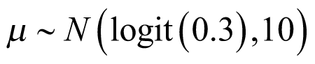
where the was the pooled mean effect across cancer types and was the SD qualifying the heterogeneity between cancer types. A normal weakly informative prior distribution with a mean probability of response of 30%, (or −0.8473 on the logit scale) which was considered as a clinically meaning full response rate, but other values can be used based on the context, a pessimist response rate of 5% for example. A variance of 10 on the logit scale with high uncertainty around the mean was selected. As discussed previously, a half-t prior with 1 degree of freedom and scale parameter of 10 (precision of 0.01) was selected, assuming limited information-sharing across cancer types. The prior distributions used in the analysis are:

The probability of response of each cancer type, , can be derived using the inverse logit function:

The model is based on Thall et al.⁷ and was estimated using a Markov chain Monte Carlo in Jags (version 4.3.0) implemented in R (version 4.1.0) using R2jags (version 0.7 to 1). For all of the analyses, a total of 5,000 burn-in iterations and 50,000 iterations were run in 4 parallel chains with a thinning rate of 10. This was necessary so that model convergence could be assessed and confirmed.

Another set of sensitivity analyses were performed using the following prior distribution with higher uncertainty (heavier tail) compared to the base analysis:

Figure 4 presents the density of priors for and . Unlike a normal distribution with a variance of 3, other distributions with variances of 10 and 100 had the mass concentrated at the extreme case of 0 and 1 in a proportion scale. The mass around 0 and 1 grew as the variance increased. For the same variance, the mass will be larger around 0 if the mean was less than logit(0.5). Although these priors had more mass at 0 and 1 and were not a sensible data-generating prior, they ensured the model was completely separated regardless of the data.²⁶ Some studies³⁸ have suggested a uniform prior distribution for , but the mass limited within the boundary with assuming larger than the boundary was not likely. The half-t prior, on the other hand, did not rule out a large heterogeneity between cancer types. The larger scale had less mass around 0. Priors used in the sensitivity analysis had larger mass around 0 and 1 for and less mass around 0 for than the base analysis.

Figure 4: Distribution Density of Various Priors for µ and σ

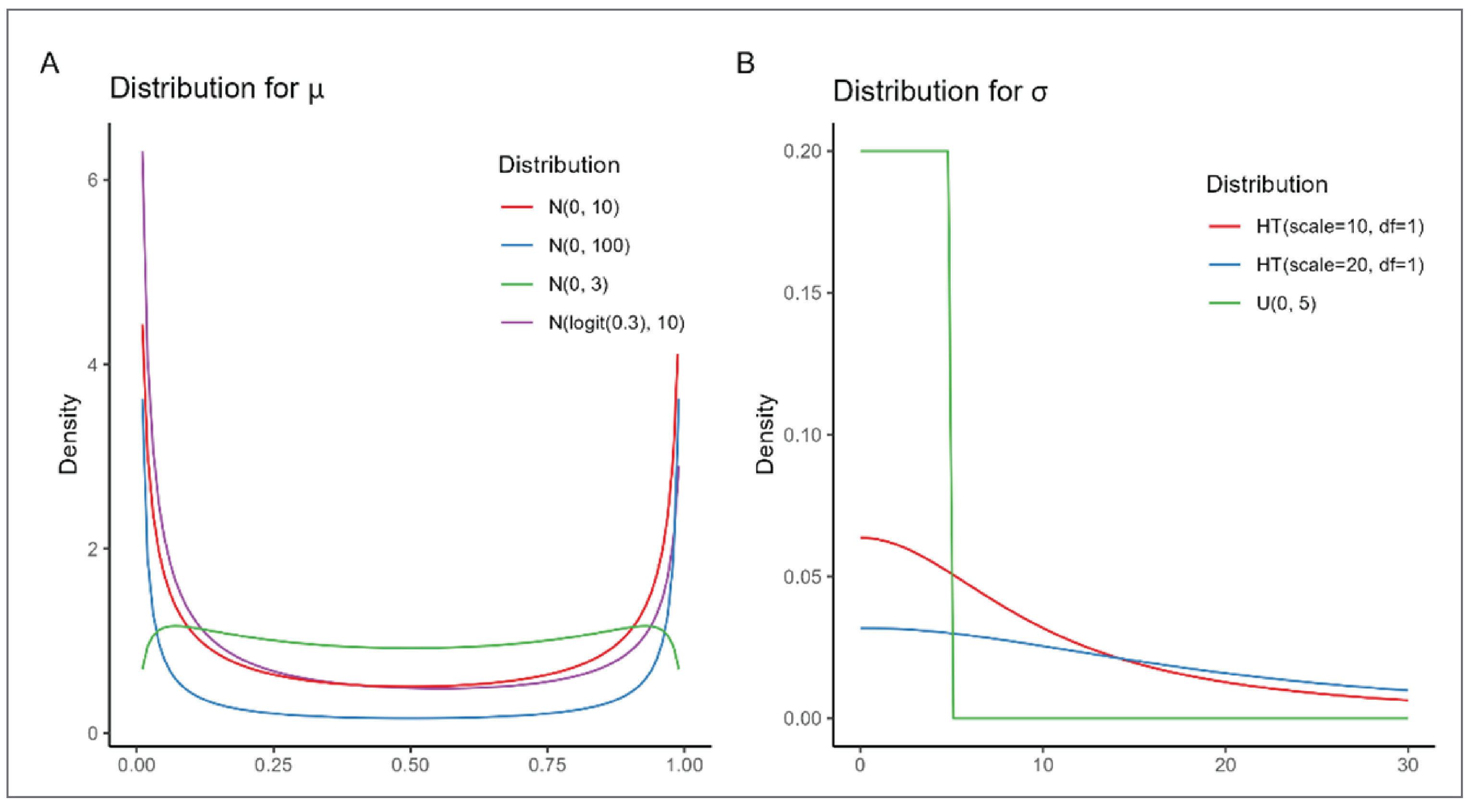
N = normal distribution; HT = half-t distribution; U = uniform distribution.

Additional Analyses

We compared the results of the BHM against 3 alternative approaches to the analysis; independent, EXNEX, and CBHM approaches were also applied.

• Independent: The independent analysis approach assumed an independent effect across cancer types and used a normal prior distribution for each cancer type, to align with the assumptions made in the BHM.

• EXNEX: A mixture of 2 exchangeable components and 1 nonexchangeable component with equal weights summing to 1 were used for all cancer types, The prior of the parameters follows a normal distribution with a mean response rate of 0.05 (low response) and 0.3 (high response) for the 2 exchangeable components and 0.15 as middles for the nonexchangeable component. The variance of the distributions was based on the formula with being the response rate.

• CBHM: For simplicity in this analysis, cancer types were clustered into 3 groups based on a k-means clustering algorithm applied on the observed proportions. Three independent BHMs were applied separately for 3 clusters after the clusters were identified. The optimal number of clusters was determined using within-cluster sums of squares and average silhouette methods. These methods measure the quality of clustering by measuring its cohesiveness. Cluster 1 includes colorectal cancer, esophageal carcinoma, pancreatic ductal adenocarcinoma (PDAC), castration-resistant prostate cancer, epithelial ovarian cancer, gastric adenocarcinoma, glioblastoma, squamous cell carcinoma of the head and neck, hepatocellular carcinoma, cervical carcinoma, and renal cell carcinoma; cluster 2 contains non–small-cell lung cancer, small-cell lung cancer, and endometrial carcinoma; and cluster 3 includes triple-negative breast cancer, metastatic urothelial cancer and HR-positive metastatic breast cancer. The prior of the parameters followed a normal distribution with mean response rates of 0.05, 0.15, and 0.3 for the 3 clusters, respectively. The same method that was used with EXNEX was used to calculate the variance of the distribution.

Economic Evaluation

We extrapolated the response rate analysis on the case study basket trial to a QALY outcome. We did this to illustrate how results from basket trials could be extended over long time horizons and eventually be used in economic evaluations, alongside costing evidence. This is not a document on the best practice of extrapolation of response rates and merely serves the purpose of illustration. As noted previously, there are multiple ways of extrapolating response rates to survival outcomes, all with their own challenges and limitations. For simplicity, in this simulation we relied on the landmark method. The landmark method estimates OS based on the response status assuming it is a perfect surrogate end point for OS. In almost all cases, this is not a plausible assumption because response is rarely capable of independently predicting mean life expectancy. This model consists of 3 mutually exclusive health states: progression-free disease, progressed disease, and death.²⁰ A normal distribution is assumed around expected survival time and a beta distribution for expected health utility of responders and nonresponders, with the hypothetical parameters given in Table 2. For simplicity, it is further assumed that all patients will progress before death. We adopted the Bayesian paradigm, and hence the complete posterior distribution was used to estimate QALYs and propagate uncertainty from response rates to QALYs.

Table 2: Assumed Hypothetical Input Parameters Included in the Economic Model

Parameters	Mean (SD)
Life expectancy
Mean time to disease progression
Responders	24 (1.2) months
Nonresponders	6 (0.3) months
Mean time from progression to death	6 (0.3) months
Utilities
Progression-free disease	0.79 (0.05)
Progressed disease	0.64 (0.035)

SD = standard deviation.

Results

Response Rate

As shown in Figure 5, the estimated overall response rate of the BHM across cancer types was 11.3% (95% CrI, 3.6% to 20.0%), lower than the pooled analysis of observed response rates (21.1%; 95% CrI, 17.4% to 25.0%). The estimated overall mean response rates and their CrIs for 2 exchangeable components of the EXNEX model were larger than the BHM. The mean overall estimated response rate was not available for the nonexchangeable component due to the independence assumption. The estimated overall mean response rates of the 3 clusters of the CBHM varied from 4.2% to 33.1% (Table 3).

Figure 5: Posterior and Predictive Distribution of the Overall Response Rate

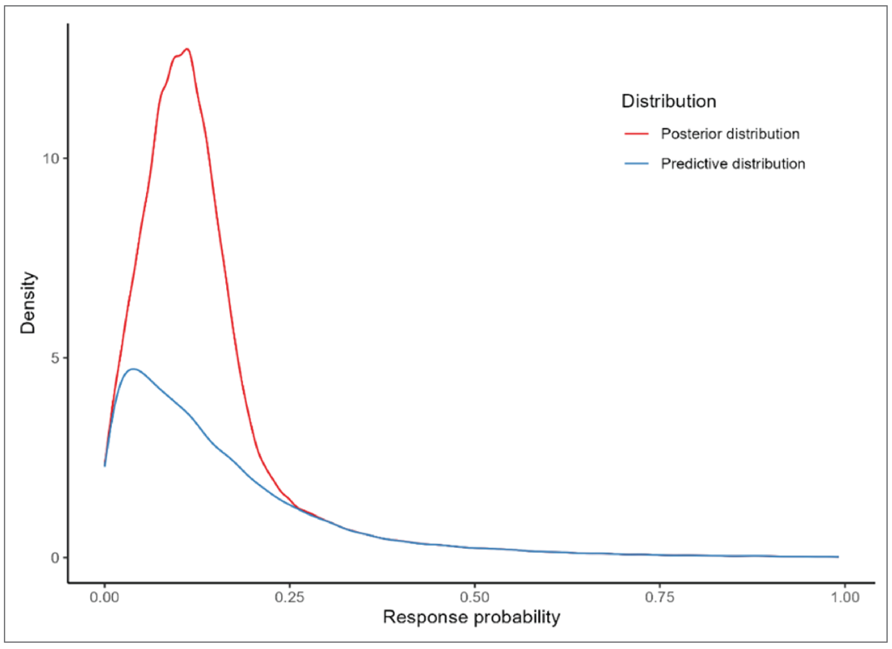
Table 3: Estimated Response Rate Across Cancer Type and Predicted Response Rate of Unpresented Cancer Type

Method	Estimated overall mean, % (95% CrI)	Predicted, % (95% CrI)
Pooled	21.1 (17.4 to 25.0)	—
BHM	11.3 (3.6 to 20.0)	15.8 (0.6 to 59.3)
EXNEX
Exchangeable component 1	18.1 (1.3 to 50.7)	23.3 (0.0 to 99.4)
Exchangeable component 2	8.8 (0.0 to 45.7)	16.5 (0.0 to 99.9)
CBHM
Cluster 1	2.3 (0.1 to 6.8)	4.2 (0.0 to 22.9)
Cluster 2	19.0 (5.4 to 43.3)	21.1 (1.2 to 76.5)
Cluster 3	32.0 (15.3 to 53.4)	33.1 (5.9 to 76.2)

BHM = Bayesian hierarchical model; CBHM = clustered Bayesian hierarchical model; CrI = credible interval; EXNEX = exchangeability-nonexchangeability.

In the BHM model, the posterior mean of , which shows between cancer type heterogeneity, was 1.18 (95% CrI, 0.49 to 2.42). Figure 6 shows the distribution of prior and posterior distributions of . The figure suggested that the prior distribution was weakly informative and appeared reasonable because the prior distribution has a substantially heavier tail than the posterior distribution.

Figure 6: Prior and Posterior Distribution of the Parameter Measuring Between Cancer Type Heterogeneity and the Standard Deviation σ of BHM

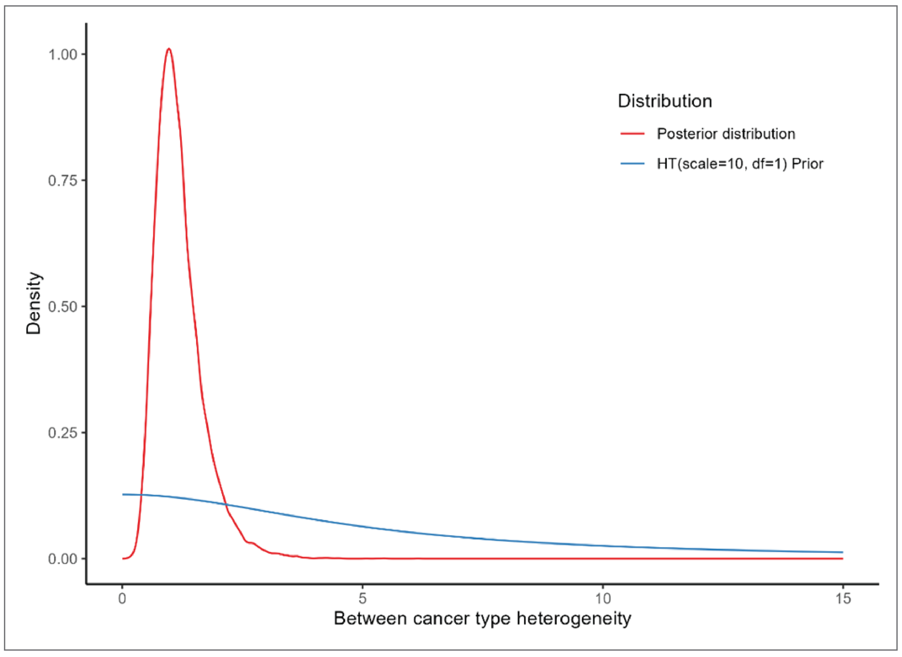
BHM = Bayesian hierarchical model; df = degrees of freedom; HT = half-t distribution.

Naturally, given the absence of any observed evidence, the predicted response rates of unobserved cancer types are inherently more uncertain. For the BHM the mean prediction was 15.8%, with a CrI of 0.6% to 59.3%. Although the predicted response rate was 23.3% and 16.5% for the 2 components of EXNEX model, the CrI was very wide with a lower bound of 0% to the upper bound as high as 99%. The predicted response rate of unpresented cancer type in 3 clusters of the CBHM ranged from 4.2% to 33.1%, but the CrI was wider than the BHM with upper bound around 76% (Table 3). These wide CrIs illustrate the importance of prior distribution assumptions around predicting response rates and in consequence intuitively wide communication of the magnitude of uncertainty to decision-makers as well as careful consideration of how this uncertainty impacts results that guide decision-making. At minimum, extensive sensitivity analysis on the expected effectiveness of treatment on unobserved cancer types is required. This sensitivity analysis can be performed by the sponsor by assuming more conservative (pessimistic) priors on the effectiveness of the unobserved cancer types or by CADTH by choosing different effectiveness assumptions for these cancer types. The former would be preferrable since the assumptions can be more seamlessly embedded in the modelling process instead of modifying the use of effectiveness estimates ex ante.

The estimated probabilities of response for each cancer type are shown in Table 4. Comparing the estimated response rate of independent analysis with the BHM, the estimated probabilities of the response rates were shrunk toward the overall mean probabilities when information-borrowing was allowed. It was worth noting that the cancer types with small sample sizes, (e.g., hepatocellular, cervical, and renal cell carcinoma), had a larger point estimation and wider CrIs in the independent analysis compared to the BHM. The prior used in the independent analysis may have more weight on the results when the sample size was small. The BHM, on the other hand, had narrower CrIs due to borrowing information across cancer types and safeguarding to avoid extreme estimation when sample sizes were small. Cancer types with fewer patients borrowed more information than those with more patients. This is also the case with the CBHM; however, in the CBHM, shrinkage took place within each cluster.

The sensitivity analysis results for the BHM are shown in the Additional Analyses section. The changes in the response rate for different cancer types, overall mean, and predicted mean were all less than 0.4%.

Table 4: Observed and Estimated Response Rate With 95% CrI for all Cancer Types

Cancer type	Observed response rate (%)	Estimated mean response rate (95% CrI)
		Independent	BHM	EXNEX	CBHM
TNBCc	36 of 108 (33.3%)	33.3 (24.9 to 42.5)	32.1 (23.6 to 41.1)	32.3 (24.0 to 41.4)	32.6 (25.1 to 40.8)
mUCc	13 of 45 (28.9%)	28.9 (16.8 to 42.5)	26.7 (15.4 to 39.9)	27.5 (16.1 to 41.0)	30.4 (19.8 to 40.7)
NSCLCb	9 of 54 (16.7%)	16.9 (8.3 to 27.9)	16.0 (8.1 to 26.0)	17.3 (8.5 to 27.8)	17.3 (9.6 to 26.5)
HR+ MBCc	17 of 54 (31.5%)	31.4 (19.9 to 44.3)	29.4 (18.5 to 41.8)	30.0 (19.2 to 42.7)	31.6 (22.0 to 41.9)
SCLCb	11 of 62 (17.7%)	17.8 (9.5 to 28.0)	17.1 (9.4 to 26.9)	18.1 (9.7 to 28.2)	17.8 (10.3 to 26.8)
CRCa	1 of 31 (3.2%)	4.1 (0.3 to 12.7)	6.0 (0.8 to 15.4)	4.5 (0.3 to 14.5)	2.8 (0.3 to 8.4)
Esophageal carcinomaa	1 of 19 (5.3%)	6.4 (0.4 to 20.0)	8.1 (1.1 to 20.4)	7.2 (0.4 to 22.3)	3.5 (0.3 to 11.5)
Endometrialb	4 of 18 (22.2%)	22.4 (7.0 to 43.0)	19.5 (6.9 to 37.6)	21.5 (7.3 to 40.2)	19.8 (9.1 to 36.4)
PDACa	0 of 16 (0.0%)	2.4 (0.0 to 12.2)	5.7 (0.2 to 17.5)	2.4 (0.0 to 13.3)	2.2 (0.0 to 7.7)
CRPCa	1 of 11 (9.1%)	10.7 (0.7 to 32.7)	11.0 (1.5 to 28.1)	11.6 (0.8 to 31.1)	4.4 (0.4 to 17.3)
EOCa	0 of 8 (0.0%)	4.3 (0.0 to 21.9)	7.7 (0.3 to 23.6)	4.5 (0.0 to 22.9)	2.5 (0.0 to 9.6)
Gastric adenocarcinomaa	0 of 5 (0.0%)	6.0 (0.0 to 31.2)	9.2 (0.4 to 28.6)	6.2 (0.0 to 29.3)	2.7 (0.0 to 10.5)
GBMa	0 of 3 (0.0%)	8.8 (0.0 to 45.7)	10.6 (0.4 to 34.5)	8.4 (0.0 to 36.6)	3.0 (0.0 to 12.7)
SCCHNa	0 of 4 (0.0%)	7.2 (0.0 to 37.5)	9.7 (0.4 to 31.3)	7.1 (0.0 to 31.8)	2.8 (0.0 to 11.5)
Hepatocellulara	0 of 2 (0.0%)	11.9 (0.0 to 59.6)	11.7 (0.4 to 39.2)	10.2 (0.0 to 44.7)	3.0 (0.0 to 13.2)
Cervicala	0 of 1 (0.0%)	18.0 (0.0 to 81.2)	13.2 (0.5 to 46.4)	12.9 (0.0 to 61.5)	3.3 (0.0 to 15.2)
RCCa	0 of 1 (0.0%)	18.3 (0.0 to 81.6)	13.3 (0.5 to 46.1)	13.4 (0.0 to 62.4)	3.4 (0.0 to 15.9)

BHM = Bayesian hierarchical model; CBHM = clustered Bayesian hierarchical model; CrI = credible interval; CRC = colorectal cancer; CRPC = castrate-resistant prostate cancer; EOC = epithelial ovarian cancer; EXNEX = exchangeability-nonexchangeability; GBM = glioblastoma multiforme; HR+ = hormone receptor-positive; MBC = metastatic breast cancer; mUC = metastatic urothelial cancer; PDAC = pancreatic ductal adenocarcinoma; RCC = renal cell carcinoma; SCCHN = squamous cell carcinoma of the head and neck; SCLC = small-cell lung cancer; TNBC = triple-negative breast cancer.

^aThis cancer type was included in cluster 1.

^bThis cancer type was included in cluster 2.

^cThis cancer type was included in cluster 3.

Economic Evaluation

Most of the basket trials are single-arm studies, which makes it imperative to construct a comparator for the comparative effectiveness analysis. We did not perform a comparative analysis in the section for the simplicity reason, methods on comparator discussed in the later section. Table 5 presents the results of extrapolation of the surrogate output from the basket trial to QALYs using the information on expected survival and utility within the assumed health states as provided in Table 2. The estimated incremental QALY was slightly higher in the pooled analysis (0.97; 96% CrI, 0.82 to 1.122) compared to the BHM approach (0.85; 95% CrI, 0.68 to 1.02). The predicted incremental QALYs was 0.90 (95% CrI 0.65 to 1.43) in the BHM for an unpresented cancer type. The predicted QALYs of 2 exchangeable components were higher in the EXNEX approach with wider CrI compared to the BHM, while the QALYs were 0.77 (95% CrI, 0.61 to 1.01), 0.97 (95% CrI, 0.69 to 1.62), and 1.11 (95% CrI, 0.78 to 1.62) in 3 clusters of the CBHM (Table 5).

Table 5: Estimated Overall Mean Incremental QALYs Across Cancer Type and Predicted Incremental QALYS of Unpresented Cancer Types

Method	Estimated overall mean QALYs (95% CrI)	Predicted QALYs (95% CrI)
Pooled	0.97 (0.82 to 1.12)	—
BHM	0.85 (0.68 to 1.02)	0.90 (0.65 to 1.43)
EXNEX
Exchangeable component 1	0.93 (0.67 to 1.32)	0.99 (0.65 to 1.87)
Exchangeable component 2	0.82 (0.61 to 1.28)	0.91 (0.61 to 1.92)
CBHM
Cluster 1	0.74 (0.60 to 0.89)	0.77 (0.61 to 1.01)
Cluster 2	0.94 (0.73 to 1.24)	0.97 (0.69 to 1.62)
Cluster 3	1.10 (0.86 to 1.38)	1.11 (0.78 to 1.62)

CBHM = clustered Bayesian hierarchical model; CrI = credible interval; EXNEX = exchangeability-nonexchangeability; QALY = quality-adjusted life year.

The estimated incremental QALYs by cancer type are presented in Table 6. The estimated QALYs varied between cancer types, but different methods yield comparable results. This is primarily due to the fact that even though on a relative scale the differences on response rates were large for some cancer types (e.g., for PDAC, the BHM estimated a response rate that was 3 times larger than the independent approach [7.7% versus 2.4%]), on an absolute scale the response rate difference was quite small (e.g., PDAC = 5.3%). Therefore, the absolute difference in response was so small that generally we did not observe large differences in estimated QALYs between methods. It is unclear to what extend this is a generalizable outcome and it will most definitely vary based on the impact of factors such as response on survival and the baseline risk of response. Generally, the more predictive response is of OS, the larger the impact of the method on the outcomes. Also, the more the heterogeneity between cancer types the greater the impact.

Table 6: Estimated Incremental QALYs by Cancer Type and Models

Cancer type	Independent (95% CrI)	BHM (95% CrI)	EXNEX (95% CrI)	CBHM (95% CrI)
TNBCc	1.11 (0.93 to 1.30)	1.10 (0.92 to 1.28)	1.10 (0.92 to 1.28)	1.10 (0.93 to 1.28)
mUCc	1.06 (0.86 to 1.28)	1.03 (0.84 to 1.25)	1.04 (0.84 to 1.26)	1.08 (0.89 to 1.27)
NSCLCb	0.92 (0.74 to 1.11)	0.91 (0.74 to 1.09)	0.92 (0.75 to 1.11)	0.92 (0.76 to 1.10)
HR+ MBCc	1.09 (0.89 to 1.30)	1.06 (0.87 to 1.27)	1.07 (0.88 to 1.28)	1.09 (0.91 to 1.28)
SCLCb	0.93 (0.75 to 1.11)	0.92 (0.75 to 1.10)	0.93 (0.76 to 1.11)	0.93 (0.77 to 1.10)
CRCa	0.76 (0.61 to 0.93)	0.79 (0.63 to 0.96)	0.77 (0.61 to 0.94)	0.75 (0.61 to 0.90)
Esophageal carcinomaa	0.79 (0.63 to 1.00)	0.81 (0.64 to 1.01)	0.80 (0.63 to 1.02)	0.76 (0.61 to 0.92)
Endometrialb	0.98 (0.74 to 1.27)	0.95 (0.74 to 1.21)	0.97 (0.75 to 1.24)	0.95 (0.76 to 1.19)
PDACa	0.74 (0.60 to 0.92)	0.78 (0.62 to 0.97)	0.74 (0.59 to 0.92)	0.74 (0.60 to 0.89)
CRPCa	0.84 (0.64 to 1.13)	0.85 (0.66 to 1.09)	0.85 (0.65 to 1.12)	0.77 (0.61 to 0.96)
EOCa	0.77 (0.60 to 1.00)	0.81 (0.63 to 1.03)	0.77 (0.60 to 1.01)	0.75 (0.60 to 0.90)
Gastric adenocarcinomaa	0.79 (0.61 to 1.11)	0.82 (0.63 to 1.09)	0.79 (0.60 to 1.09)	0.75 (0.60 to 0.91)
GBMa	0.82 (0.61 to 1.26)	0.84 (0.63 to 1.15)	0.81 (0.61 to 1.17)	0.75 (0.60 to 0.93)
SCCHNa	0.80 (0.61 to 1.18)	0.83 (0.63 to 1.11)	0.80 (0.60 to 1.12)	0.75 (0.60 to 0.92)
Hepatocellulara	0.86 (0.61 to 1.44)	0.85 (0.64 to 1.20)	0.84 (0.61 to 1.26)	0.75 (0.60 to 0.93)
Cervicala	0.93 (0.62 to 1.68)	0.87 (0.64 to 1.27)	0.87 (0.61 to 1.45)	0.76 (0.61 to 0.94)
RCCa	0.93 (0.62 to 1.68)	0.87 (0.64 to 1.28)	0.87 (0.62 to 1.45)	0.76 (0.61 to 0.95)

BHM = Bayesian hierarchical model; CBHM = clustered Bayesian hierarchical model; CrI = credible interval; CRC = colorectal cancer; CRPC = castrate-resistant prostate cancer; EOC = epithelial ovarian cancer; EXNEX = exchangeability-nonexchangeability; GBM = glioblastoma multiforme; HR+ = hormone receptor-positive; MBC = metastatic breast cancer; mUC = metastatic urothelial cancer; PDAC = pancreatic ductal adenocarcinoma; RCC = renal cell carcinoma; SCCHN = squamous cell carcinoma of the head and neck; SCLC = small-cell lung cancer; TNBC = triple-negative breast cancer.

^aThis cancer type was included in cluster 1.

^bThis cancer type was included in cluster 2.

^cThis cancer type was included in cluster 3.

Additional Analyses

Impact of Excluding Cancer Types

In the main analysis, all cancer types were included in the analysis. To investigate the impact of possibly missing information on some cancer types, 2 sets of analysis were performed: 1 in which cancer types with fewer than 10 patients were excluded, and 1 in which cancer types were excluded sequentially while keeping all remaining cancer types (i.e., a leave-one-out analysis). All other analysis settings were the same as described in the main section. Results from independent analysis and the BHM were also presented here as a reference.

Response Rate

When cancer types with sample sizes comprising fewer than 10 patients were excluded, the change in the estimated response rate was modest for most of the cancer types compared to analyzing all cancer types (Table 7). Response rates for CRC, PDAC, and CRPC increased when only cancer types with fewer than 10 patients were excluded from the analysis. Similarly, the estimated overall mean response rate increased from 11.3 (95% CrI, 3.6 to 20.0) in the full analysis to 15.9 (95% CrI, 6.4 to 27.1) after excluding cancer types with fewer than 10 patients (Table 8). As was the case in the main analysis, the response rate of all cancer types was pulled toward the estimated overall mean response rate.

Table 7: Observed, Estimated, and Predicted Response Rate for all Cancer Types

Cancer	Observed response rate (%)	BHMa (95% CrI)	BHM excluding cancer types with < 10 patients (95% CrI)
TNBC	36 of 108 (33.3%)	32.1 (23.6 to 41.1)	32 (23.7 to 41)
mUC	13 of 45 (28.9%)	26.7 (15.4 to 39.9)	26.9 (15.9 to 40.1)
NSCLC	9 of 54 (16.7%)	16.0 (8.1 to 26.0)	16.7 (8.6 to 26.8)
HR+ MBC	17 of 54 (31.5%)	29.4 (18.5 to 41.8)	29.5 (18.9 to 41.9)
SCLC	11 of 62 (17.7%)	17.1 (9.4 to 26.9)	17.6 (9.8 to 27.3)
CRC	1 of 31 (3.2%)	6.0 (0.8 to 15.4)	7.3 (1.2 to 17.8)
Esophageal carcinoma	1 of 19 (5.3%)	8.1 (1.1 to 20.4)	9.8 (1.6 to 23)
Endometrial	4 of 18 (22.2%)	19.5 (6.9 to 37.6)	20.5 (7.6 to 38.6)
PDAC	0 of 16 (0.0%)	5.7 (0.2 to 17.5)	7.7 (0.5 to 20.8)
CRPC	1 of 11 (9.1%)	11.0 (1.5 to 28.1)	13 (2.3 to 30.5)
EOC	0 of 8 (0.0%)	7.7 (0.3 to 23.6)	—
Gastric adenocarcinoma	0 of 5 (0.0%)	9.2 (0.4 to 28.6)	—
GBM	0 of 3 (0.0%)	10.6 (0.4 to 34.5)	—
SCCHN	0 of 4 (0.0%)	9.7 (0.4 to 31.3)	—
Hepatocellular	0 of 2 (0.0%)	11.7 (0.4 to 39.2)	—
Cervical	0 of 1 (0.0%)	13.2 (0.5 to 46.4)	—
RCC	0 of 1 (0.0%)	13.3 (0.5 to 46.1)	—

CRC = colorectal cancer; CRPC = castrate-resistant prostate cancer; EOC = epithelial ovarian cancer; GBM = glioblastoma multiforme; HR+ = hormone receptor-positive; MBC = metastatic breast cancer; mUC = metastatic urothelial cancer; PDAC = pancreatic ductal adenocarcinoma; RCC = renal cell carcinoma; SCCHN = squamous cell carcinoma of the head and neck; SCLC = small-cell lung cancer; TNBC = triple-negative breast cancer.

^aBHM results from all cancer types are presented here as a reference.

Table 8 presents the overall mean and predicted response rate, ?. As expected, overall mean and predicted response rate from the 10 cancer types analysis were larger than the all cancer types analysis, as the excluded cancer types had no response. However, the CrI was wider than the all cancer types analysis, as there were less data to borrow. There was no material difference in between cancer type heterogeneity, , between the 2 sets of analysis. The magnitude of change in the overall mean and predicted response rate depended on the sample size of the excluded cancer type. The impact of sequentially removing cancer types on the overall mean and predicted response rate was larger when the excluded cancer type had a larger sample size and when the excluded response rate was further from the mean response rate.

Table 8: Overall Mean Response Rate Across Cancer Type, Predicted Response Rate of Unpresented Cancer Type, and Between Cancer Type Heterogeneity Using the BHM

Cancer type	Overall mean response, % (95% CrI)	Predicted, % (95% CrI)	σ (95% CrI)
BHM (cancer types with < 10 patients excluded)	15.9 (6.4 to 27.1)	19.7 (1.3 to 65.2)	1.03 (0.39 to 2.24)
All cancer types	11.3 (3.6 to 20.0)	15.8 (0.6 to 9.3)	1.21 (0.49 to 2.45)
Excluded cancer typea
TNBC	9.81 (2.72 to 18.12)	14.42 (0.45 to 58.36)	1.19 (0.42 to 2.55)
mUC	9.66 (2.47 to 18.67)	14.55 (0.35 to 60.46)	1.29 (0.53 to 2.69)
NSCLC	9.88 (2.53 to 19.42)	15.77 (0.33 to 64.94)	1.39 (0.59 to 2.80)
HR+ MBC	9.83 (2.68 to 18.56)	14.35 (0.30 to 58.12)	1.24 (0.49 to 2.58)
SCLC	9.98 (2.57 to 19.37)	15.35 (0.30 to 64.25)	1.36 (0.58 to 2.81)
CRC	13.12 (4.28 to 22.43)	16.89 (0.81 to 54.83)	1.05 (0.35 to 2.38)
Esophageal carcinoma	12.07 (3.36 to 21.74)	16.63 (0.44 to 60.77)	1.20 (0.45 to 2.64)
Endometrial	9.93 (2.31 to 19.32)	15.39 (0.28, 64.71)	1.36 (0.58 to 2.85)
PDAC	13.43 (5.08 to 22.53)	16.88 (1.03 to 55.55)	1.00 (0.38 to 2.08)
CRPC	11.14 (2.93 to 20.84)	16.07 (0.41 to 65.41)	1.27 (0.51 to 2.68)
EOC	12.53 (4.44 to 21.64)	16.59 (0.77 to 58.24)	1.11 (0.46 to 2.27)
Gastric adenocarcinoma	11.95 (3.91 to 21.11)	16.34 (0.57 to 60.03)	1.16 (0.47 to 2.49)
GBM	11.87 (3.72 to 21.02)	16.40 (0.62 to 60.92)	1.16 (0.47 to 2.37)
SCCHN	12.07 (3.94 to 21.24)	16.72 (0.61 to 63.01)	1.16 (0.46 to 2.34)
Hepatocellular	11.58 (3.68 to 20.65)	16.34 (0.61 to 61.64)	1.18 (0.49 to 2.44)
Cervical	11.38 (3.63 to 20.30)	15.92 (0.56 to 59.01)	1.20 (0.50 to 2.44)
RCC	11.40 (3.68 to 20.17)	16.37 (0.63 to 61.49)	1.18 (0.47 to 2.37)

CRC = colorectal cancer; CRPC = castrate-resistant prostate cancer; EOC = epithelial ovarian cancer; GBM = glioblastoma multiforme; HR+ = hormone receptor-positive; MBC = metastatic breast cancer; mUC = metastatic urothelial cancer; PDAC = pancreatic ductal adenocarcinoma; RCC = renal cell carcinoma; SCCHN = squamous cell carcinoma of the head and neck; SCLC = small-cell lung cancer; TNBC = triple-negative breast cancer.

^aOverall and predicted response rate after the exclusion of the corresponding cancer type.

Economic Evaluation – Additional Analyses

Table 9 presents the estimated incremental QALYs by cancer types. Similar to the main analysis results, the estimated QALYs varied between cancer types. The estimated QALYs from the analysis where cancer types with fewer than 10 patients were excluded were similar to the all cancer types results. The estimated overall mean QALYs and predicted QALYs were higher when cancer types with less than 10 patients were excluded in the analysis (Table 10).

Table 9: Estimated and Predicted Incremental QALYs by Cancer Type and Models

Cancer type	BHMa (95% CrI)	BHM excluding cancer types with < 10 patients (95% CrI)
TNBC	1.10 (0.92 to 1.28)	1.09 (0.92 to 1.28)
mUC	1.03 (0.84 to 1.25)	1.03 (0.84 to 1.25)
NSCLC	0.91 (0.74 to 1.09)	0.91 (0.74 to 1.09)
HR+ MBC	1.06 (0.87 to 1.27)	1.06 (0.87 to 1.27)
SCLC	0.92 (0.75 to 1.10)	0.92 (0.75 to 1.11)
CRC	0.79 (0.63 to 0.96)	0.80 (0.64 to 0.98)
Esophageal carcinoma	0.81 (0.64 to 1.01)	0.83 (0.65 to 1.04)
Endometrial	0.95 (0.74 to 1.21)	0.96 (0.75 to 1.22)
PDAC	0.78 (0.62 to 0.97)	0.80 (0.63 to 1.01)
CRPC	0.85 (0.66 to 1.09)	0.87 (0.67 to 1.11)
EOC	0.81 (0.63 to 1.03)	—
Gastric adenocarcinoma	0.82 (0.63 to 1.09)	—
GBM	0.84 (0.63 to 1.15)	—
SCCHN	0.83 (0.63 to 1.11)	—
Hepatocellular	0.85 (0.64 to 1.20)	—
Cervical	0.87 (0.64 to 1.27)	—
RCC	0.87 (0.64 to 1.28)	—

CRC = colorectal cancer; CRPC = castrate-resistant prostate cancer; EOC = epithelial ovarian cancer; GBM = glioblastoma multiforme; HR+ = hormone receptor-positive; MBC = metastatic breast cancer; mUC = metastatic urothelial cancer; PDAC = pancreatic ductal adenocarcinoma; RCC = renal cell carcinoma; SCCHN = squamous cell carcinoma of the head and neck; SCLC = small-cell lung cancer; TNBC = triple-negative breast cancer.

^aBHM results from all cancer types are presented here as a reference.

Table 10: Overall Incremental QALYs Across Cancer Type and Predicted Incremental QALYs of Unpresented Cancer Type Using BHM

Cancer type	Overall mean QALYs (95% CrI)	Predicted QALYs (95% CrI)
BHM (cancer types with < 10 patients excluded)	0.90 (0.72 to 1.10)	0.95 (0.67 to 1.50)
All cancer types	0.85 (0.68 to 1.02)	0.91 (0.66 to 1.44)
Excluded cancer typea
TNBC	0.83 (0.67 to 1.00)	0.89 (0.64 to 1.40)
mUC	0.83 (0.67 to 1.01)	0.89 (0.65 to 1.42)
NSCLC	0.83 (0.67 to 1.01)	0.90 (0.64 to 1.49)
HR+ MBC	0.83 (0.67 to 1.01)	0.89 (0.64 to 1.42)
SCLC	0.84 (0.67 to 1.01)	0.90 (0.65 to 1.47)
CRC	0.87 (0.70 to 1.05)	0.92 (0.66 to 1.38)
Esophageal carcinoma	0.86 (0.68 to 1.04)	0.91 (0.65 to 1.45)
Endometrial	0.83 (0.67 to 1.01)	0.90 (0.64 to 1.49)
PDAC	0.87 (0.70 to 1.06)	0.91 (0.66 to 1.38)
CRPC	0.85 (0.67 to 1.03)	0.90 (0.64 to 1.49)
EOC	0.86 (0.70 to 1.04)	0.91 (0.66 to 1.41)
Gastric adenocarcinoma	0.86 (0.69 to 1.03)	0.91 (0.65 to 1.46)
GBM	0.85 (0.69 to 1.03)	0.91 (0.65 to 1.46)
SCCHN	0.86 (0.69 to 1.04)	0.91 (0.65 to 1.46)
Hepatocellular	0.85 (0.69 to 1.03)	0.91 (0.65 to 1.47)
Cervical	0.85 (0.68 to 1.03)	0.90 (0.65 to 1.42)
RCC	0.85 (0.69 to 1.03)	0.91 (0.66 to 1.48)

CRC = colorectal cancer; CRPC = castrate-resistant prostate cancer; EOC = epithelial ovarian cancer; GBM = glioblastoma multiforme; HR+ = hormone receptor-positive; MBC = metastatic breast cancer; mUC = metastatic urothelial cancer; PDAC = pancreatic ductal adenocarcinoma; RCC = renal cell carcinoma; SCCHN = squamous cell carcinoma of the head and neck; SCLC = small-cell lung cancer; TNBC = triple-negative breast cancer.

^aEstimated and predicted QALYs after the exclusion of the corresponding cancer type.

Sensitivity Analysis Result of BHM

Table 11: Estimated Response Rate for all Cancer Types in Base and Sensitivity Analysis

Cancer type	Base BHM (95% CrI)	Sensitivity BHM (95% CrI)
Estimated overall mean response, %	11.3 (3.6 to 20.0)	11.0 (3.1 to 19.8)
Predicted response, %	15.8 (0.6 to 59.3)	15.7 (0.5 to 59.3)
All cancer types
TNBC	32.1 (23.6 to 41.1)	32.1 (23.6 to 41.1)
mUC	26.7 (15.4 to 39.9)	26.7 (15.5 to 40.1)
NSCLC	16.0 (8.1 to 26.0)	16.1 (8.1 to 26.2)
HR+ MBC	29.4 (18.5 to 41.8)	29.3 (18.4 to 41.8)
SCLC	17.1 (9.4 to 26.9)	17.1 (9.3 to 26.9)
CRC	6.0 (0.8 to 15.4)	5.9 (0.8 to 15.0)
Esophageal carcinoma	8.1 (1.1 to 20.4)	8.0 (1.0 to 20.8)
Endometrial	19.5 (6.9 to 37.6)	19.5 (6.7 to 37.9)
PDAC	5.7 (0.2 to 17.5)	5.6 (0.2 to 17.3)
CRPC	11.0 (1.5 to 28.1)	10.9 (1.4 to 28.1)
EOC	7.7 (0.3 to 23.6)	7.6 (0.3 to 23.8)
Gastric adenocarcinoma	9.2 (0.4 to 28.6)	8.9 (0.3 to 28.3)
GBM	10.6 (0.4 to 34.5)	10.4 (0.3 to 33.8)
SCCHN	9.7 (0.4 to 31.3)	9.4 (0.3 to 30.5)
Hepatocellular	11.7 (0.4 to 39.2)	11.5 (0.4 to 39.0)
Cervical	13.2 (0.5 to 46.4)	13.0 (0.4 to 45.8)
RCC	13.3 (0.5 to 46.1)	12.9 (0.4 to 45.4)

CRC = colorectal cancer; CRPC = castrate-resistant prostate cancer; EOC = epithelial ovarian cancer; GBM = glioblastoma multiforme; HR+ = hormone receptor-positive; MBC = metastatic breast cancer; mUC = metastatic urothelial cancer; PDAC = pancreatic ductal adenocarcinoma; RCC = renal cell carcinoma; SCCHN = squamous cell carcinoma of the head and neck; SCLC = small-cell lung cancer; TNBC = triple-negative breast cancer.

Appendix 2: Appraisal of BHMs Used in Economic Evaluations

Note that this appendix has not been copy-edited.

There are multiple factors to consider when appraising an economic evaluation that incorporates evidence from a BHM. The strength of the underlying trial evidence and the methods used to integrate it into the economic model will have a meaningful effect on the level of uncertainty surrounding the model’s estimated costs and outcomes. The following list is provided for researchers to consider when designing models that use a BHM, and for analysts when appraising them.

Table 12: Appraisal of BHMs Used in Economic Evaluations

BHM = Bayesian Hierarchical Model; HTA = health technology assessment; MAIC = matching-adjusted indirect comparison; MCMC = Markov chain Monte Carlo; vs. = versus.

Appendix 3: Terminology

Note that this appendix has not been copy-edited.

Table 13: Terminology